IV. Long-Run Cost
In the long run, a rm can vary the level of all resources so both labor and capital are
variable factors. As a result, in the long run all costs are variable costs.
The Production Function
The production function determines the behavior of long run costs.
A rm’s production function typically exhibits diminishing returns to capital as well
as diminishing returns to labor. The marginal product of capital is the change in total
product divided by the change in capital when the quantity of labor is held constant.
Holding constant the quantity of employment, after some level of output the rm will
have diminishing returns to capital—the marginal product of capital decreases as
more capital is used.
Short-Run Cost and Long-Run Cost
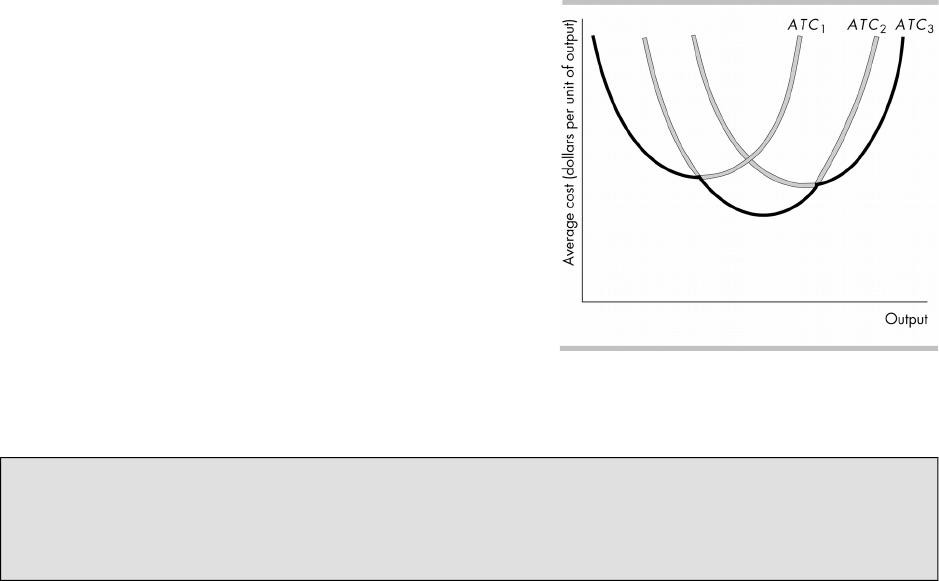
In the long run, a rm can use di#erent plant sizes. Each plant size has a di#erent
short-run ATC curve. Each short-run ATC curve is U-shaped and the larger the plant
size, the greater is the output at which the
average total cost is a minimum.
The gure illustrates three average total cost
curves for three plant sizes. ATC1 pertains to
the smallest plant size and ATC3 to the
largest.
The Long-Run Average Cost Curve
The long-run average cost curve, LRAC,
is the relationship between the lowest
attainable average total cost and output
when both the plant size and labor are
varied. This curve is derived from the
short-run average total cost curves. It shows
the lowest average total cost to produce a
given level of output. In the gure, the LRAC curve is the darkened parts of the three
short-run ATC curves.
The LRAC curve is a planning curve. Once the rm chooses a plant size, then it
operates on the short-run costs curves associated with that plant size.
An Economics in Action case describes why a rm in the auto industry might have capital
equipment that is not fully used. The rm is producing at a point on its short-run average
total cost curve that is not the minimum of the short-run average cost curve, so the rm
has under–utilized capital. But the production point is on the long-run average cost, so the
quantity being manufactured is produced at the minimum average total cost.
Economies and Diseconomies of Scale
Economies of scale are features of a rm’s technology that lead to falling long-run
average cost as output increases. With given factor prices, economies of scale occur
if the percentage increase in output exceeds the percentage increase in all factors of
production. The long-run average cost curve slopes downward in this range of
output. The main source of economies of scale is greater specialization of both labor
and capital.
Constant returns to scale are features of a rm’s technology that lead to
constant long-run average cost as output increases. With given factor prices,
economies of scale occur if the percentage increase in output equals the percentage

increase in all factors of production. The long run average cost curve is horizontal in
this range of output.
Diseconomies of scale are features of a rm’s technology that lead to rising
long-run average cost as output increases. With given factor prices, economies of
scale occur if the percentage increase in output is less than the percentage increase
in all factors of production. The long run average cost curve slopes upward in this
range of output.
The minimum ecient scale is the smallest quantity of output at which the
long-run average cost curve reaches its lowest level.
Concepts are important, not just the formulas. Make good use of the glossary of
productivity and cost terms provided in Table 11.2 in the text, but don’t get mired down in
reciting productivity and cost measure denitions! Students must learn the denitions, but
they are secondary to the concepts they dene and the insights they bring. Stand back
from the details of this chapter and be sure that your students learn two big ideas.
A rm’s lowest production costs depend on the manager’s exibility to choose the level
of all factors. This 2exibility enables rm managers to produce at a lower cost in the
long run than in the short run when some factors are xed.
In the short run, with one or more xed factors, production costs vary with output in a
predictable way because they are directly linked to measures of factor productivity.
When does the rm actually reach the “long run”? Think of the long run as a
window of opportunity in which rms get to re-make decisions. If things are going well,
rms may be re-making decisions regularly and extending xed inputs on a regular basis.
But if things are going poorly, the window in which a lease can be broken or a contract not
renewed will be pressing. Point out to the students that the long-run average cost curve
yields the lowest average cost of production possible when plant size is free to change.
Once a rm commits to a specic plant size, it is locked into a specic short run cost curve
conguration. Any signicant departure from the range of output per period that best suits
that conguration means the rm will incur higher short-run average total costs than it
would have had it chosen a more appropriate plant size. If faulty market analysis or
unexpected changes in market conditions cause a rm to commit to a plant that is too
small (or too large) when the required range of production is actually relatively high (or
relatively low), then the rm will suddenly be locked into a much less competitive
production cost situation with potentially dire economic consequences. If the rm’s
competitors chose their plant size more wisely, the rm might have a tough time surviving!
Who is successful in the long run may depend on decisions to get bigger or smaller that
wound up being correct as market conditions changed.
Experiment: Learn about production by producing. This chapter is one more place
where an in-class experiment has a huge payo# in student comprehension. This 30 minute
experiment teaches students about product curves and production cost measures. It
motivates the students to go beyond memorizing the cost and productivity denitions by
getting them directly involved with generating their own data as well as productivity and
cost measures. This fun exercise will illustrate the concept of diminishing returns to labor
as well as how short-run productivity measures and production cost measures are related.
Factors: Capital: A medium-sized table (the class must have an unobstructed view of
it), tear–o# scratch pads with about 500 sheets of paper, a fully loaded stapler, and a
back-up stapler (also fully loaded). Labor: Provided by your students.
The Task: To produce “widgets.” A widget is a piece of paper, torn from a pad, folded
twice very carefully so that the corners of the paper align, and stapled. (The rst fold

bisects the paper along its long side and the second fold is at right angles to the rst.)
Once folded, it is stapled to hold the folds in place. A widget is fragile and breaks if it
falls o# the table.
The Pre-Experiment Stage: Hire a manager from your class and appoint an auditor.
Get the manager to hire a quality controller, an accountant, and some workers. Tell the
manager that he must produce widgets as e<ciently as possible and that he can
discuss the process with his workers and with the class.
The Experiment: A “work day” lasts for 1 minute. Get the class to keep time. On day
1, have one worker produce widgets. On day 2, have two workers produce widgets, and
so on. You’ll probably run for 10 to 12 days before you get to almost zero marginal
product. Record the inputs and outputs. Have some fun with quality control, shirking,
and cheating. The auditor must ensure that old widgets and partly made widgets don’t
get used in a subsequent day. Each day must start clean.
The Assignment (Stage 1): Have the students to calculate marginal product and
average product from the total product numbers that you’re recorded. Get them to
make graphs of the total product, marginal product, and average product curves. Get
them to describe the curves and to explain their similarities with and di#erences to the
curves for sweater production in the textbook.
The Assignment (Stage 2). Use the data from your widget production experiment
and give the students gures for the cost of the capital and the wage rate of a worker.
(Make up the numbers—any will do.) Tell the students to calculate total cost, marginal
cost, and average cost. Get them to make graphs of the total cost, marginal cost, and
average cost curves. Get them to describe the curves and to explain their similarities
with and di#erences to the curves for sweaters in the textbook. (This assignment and
the previous one make an outstanding assignment for credit.)
The Experiment Extended. If you have the time, duplicate the capital of the rst
experiment and repeat all its steps. You should generate a horizontal LRAC. Get the
class to think about what would have to happen in the context of this experiment to get
economies of scale and diseconomies of scale.
Economics in the News discusses Starbucks’ cost curves and describes how adding
additional stores can move the rm downward along its long-run average cost curve and
thereby lower its average total costs.
Additional Problems
1. Charlie’s Chocolates total product schedule is
in the table.
a. Draw the total product curve.
b. Calculate the average product of labor and
draw the average product curve.
c. Calculate the marginal product of labor and
draw the marginal product curve.
d. What is the relationship between the average
product and marginal product when Charlie’s
Chocolates produces (i) less than 276 boxes
a day and (ii) more than 276 boxes a day?
Labor
(workers per
day)
Output
(boxes per
day)
1 12
2 24
3 48
4 84
5 121
6 192
7 240
8 276
9 300
10 312

2. In problem 1, the price of labor is $50 per day, and total xed costs are $50
per day.
a. Calculate total cost, total variable cost, and total xed costs for each level
of output and draw the short-run total cost curves.
b. Calculate average total cost, average xed cost, average variable cost, and
marginal cost at each level of output and draw the short-run average and
marginal cost curves.
3. In problem 2, suppose that the price of labor increases to $70 per day. Explain
what changes occur to the short-run average and marginal cost curves?
4. In problem 2, Charlie’s Chocolates buys a second plant and now the total
product of each quantity of labor doubles. The total xed cost of operating
each plant is $50 a day. The wage rate is $50 a day.
a. Set out the average total cost curve when Charlie’s operates two plants.
b. Draw the long-run average cost curve.
c. Over what output range is it e<cient to operate one plant and two plants?
5. The table shows the
production function
of Mario’s
Pizza-to-Go. Mario
must pay $100 a day
for each oven he
rents and $75 a day
for each kitchen
hand he hires
a. Find and graph the average total cost curve for each plant size.
b. Draw Mario’s long-run average cost curve.
c. Over what output range does Mario experience economies of scale?
d. Explain how Mario uses his long-run average cost curve to decide how many
ovens to rent.
S o l u t i o n s t o A d d i t i o n a l P r o b l e m s
1. a. To draw the total product curve measure labor on the x-axis and output on the
y-axis. The total product curve is upward sloping.
b. The average product of labor is equal to total product divided by the quantity of
labor employed. For example, when 3 workers are employed, they produce 48 boxes
a day, so average product is 16 boxes per worker. The average product curve is
upward sloping when the number of workers is between 1 and 8, but it becomes
downward sloping when 9 and 10 workers are employed.
c. The marginal product of labor is equal to the increase in total product when an
additional worker is employed. For example, when 3 workers are employed, total
product is 48 boxes a day. When a fourth worker is employed, total product increases
to 84 boxes a day. The marginal product of going from 3 to 4 workers is 36 boxes.
The marginal product curve is upward sloping when the number of workers is
Labor
(workers
per day)
Output
(pizzas per day)
Plant 1 Plant 2 Plant 3 Plant 4
1 4 8 11 13
2 8 12 15 17
3 11 15 18 20
4 13 17 20 22
Ovens 1 2 3 4
between 1 and 6, but it becomes downward sloping when 7 or more workers are
employed.
d. (i) When Charlie’s Chocolates produces fewer than 276 boxes a day, it employs
fewer than 8 workers a day. With fewer than 8 workers a day, marginal product
exceeds average product and average product is increasing. Up to an output of
276 boxes a day, each additional worker adds more to output than the average.
Average product increases.
(ii) When Charlie’s Chocolates produces more than 276 boxes a day, it employs
more than 8 workers a day. With more than 8 workers a day, average product
exceeds marginal product and average product is decreasing. For outputs
greater than 276 boxes a day, each additional worker adds less to output than
average. Average product decreases.
2. a. Total cost is the sum of the costs of all the inputs that Charlie’s Chocolates uses in
production. Total variable cost is the total cost of the variable inputs. Total xed cost
is the total cost of the xed inputs.
For example, the total variable cost of producing 48 boxes a day is the total cost of
the workers employed, which is 3 workers at $50 a day, which equals $150. Total
xed cost is $50, so the total cost of producing 48 boxes a day is $200.
To draw the short-run total cost curves, plot output on the x-axis and the total cost
on the y-axis. The total xed cost curve is a horizontal line at $50. The total variable
cost curve and the total cost curve have shapes similar to those in Fig. 11.4, but the
vertical distance between the total variable cost curve and the total cost curve is
$50.
b. Average xed cost is total xed cost per unit of output. Average variable cost is total
variable cost per unit of output. Average total cost is the total cost per unit of output.
For example, when the rm makes 48 boxes a day: Total xed cost is $50, so average
xed cost is $1.04 per box; total variable cost is $150, so average variable cost is
$3.13 per box; and total cost is $200, so average total cost is $4.17 per box.
Marginal cost is the increase in total cost divided by the increase in output. For
example, when output increases from 24 to 48 boxes a day, total cost increases from
$150 to $200, an increase of $50. That is, the increase in output of 24 boxes
increases total cost by $50. Marginal cost is equal to $50 divided by 24 boxes, which
is $2.08 a box.
The short-run average and marginal cost curves are similar to those in Fig. 11.5.
3. The increase in the price of labor increases total variable cost and total cost but does
not change total xed cost. Average variable cost is total variable cost per unit of
output. The average variable cost curve shifts upward. Average total cost is total cost
per unit of output. The average total cost curve shifts upward. The marginal cost curve
shifts upward. Average xed cost does not change.
4. a. Total cost is the cost of all the factors of production. For example, when 3 workers are
employed they now produce 96 boxes a day. With 3 workers, the total variable cost is
$150 a day and the total xed cost is $100 a day. The total cost is $250 a day. The
average total cost of producing 96 boxes is $2.60.
b. The long-run average cost curve is made up of the lowest parts of the rm’s
short-run average total cost curves when the rm operates one plant and two plants.
The long-run average cost curve is similar to Fig. 11.8.
c. It is e<cient to operate the number of plants that has the lower average total cost of
a box of chocolates. It is e<cient to operate one plant when output is less than 48
boxes a day, and it is e<cient to operate two plants when the output is more than 48
boxes a day. Over the output range 1 to 48 boxes a week, average total cost is less
with one plant than with two, but if output exceeds 48 boxes a day, average total
cost is less with two plants than with one.
5. a. For example, the average total cost of producing a pizza when Mario rents 2 ovens
and employs 4 workers equals the total cost ($200 rent for the ovens plus $300 for
the workers) divided by the 17 pizzas produced. The average total cost equals
$500÷17, which is $29.41 a pizza. The average total cost curve is U-shaped, as in
Fig. 11.5.
b. The long-run average cost curve is similar to that in Fig. 11.8.
c. Mario experiences economies of scale at output levels of 4 to 15 pizzas a day. When
economies of scale are present, the LRAC curve slopes downward. Mario’s LRAC
curve slopes downward between the output levels of 4 to 15 pizzas a day.
d. Mario will choose the plant (number of ovens to rent) that gives him minimum
average total cost for the normal or average number of pizzas that people buy.
A d d i t i o n a l D i s c u s s i o n Q u e s t i o n s
11. Is the law of diminishing returns a result of rms hiring the best
workers rst? Students should understand that diminishing returns to labor
occur under the assumption of a homogenous work force. Emphasize that
diminishing marginal returns occur due to labor’s decreasing productivity
given a xed level of capital. The law of diminishing returns is dened in the
short run only. As the amount of capital increases, as technology changes, or
as the size of the plant increases, labor productivity can increase. If the
variable input was a herbicide or a fertilizer on a farm eld, diminishing
returns would still be observed.
2. Do increasing marginal costs result from the rising wages of workers?
Students should understand that rising marginal cost in the short run results
from diminishing marginal productivity of labor holding the wages for labor
constant. Show the students the following thought process:
Employing another labor unit increases output, but the extra output is less
than the added output from the previous labor unit (diminishing marginal
productivity).
Each labor unit costs the same to employ, so the rm is getting less
additional output for the same additional cost (constant cost of labor).
As a result, each additional unit of output is more expensive for the rm to
make than the previous units of output (rising marginal cost).
This chain of reasoning is very important because it clearly shows the linkage
from the rm’s production decisions and production constraints to its costs and
the behavior of its cost curves.
3. Fixating on xed costs. Students should be aware of how xed costs a#ect
pricing decisions made by rms:
Why are some consumer products cheaper to buy in bulk? The
students should be aware that if packaging costs comprise a signicant
proportion of the total cost of an item, then an increase in the ratio of
product to packaging lowers the cost per unit. The rm can be more
competitive and still retain protability if it passes some of the savings on
to the customer through a lower unit price.
4. Do rms produce where the ATC (or MC) curve is at its minimum?
Students frequently ask a variation of this question. Students who ask this
question should be praised because they are clearly thinking ahead and trying
to use what they are learning to better understand the real world around them.
However, you need to be clear to these students that costs are essentially half
of the picture. Firms are in business for one reason, to maximize their prot.
Prot equals revenue minus cost, so in order to maximize their prot, rms
need also to be concerned with their revenue. You can intuitively tell the
students that the next chapters “cover the revenue side of the picture” by
looking at how the market structure in which a rm competes a#ects the rm’s
revenue and hence a#ects its decisions. Firms want to minimize the cost of
producing a given level of output, but the level of output that maximizes prot
may not be at the minimum of any cost function.
5. Discuss the following in terms of xed costs, the short run and the
long run: In agricultural markets, rms hesitate to be early adopters
of new technologies embodied in new capital equipment, which can
be quite expensive. But once they are proven to increase
productivity, rms rush to adopt them and rms that don’t (or can’t)
will have di6culty surviving. Equipment is a huge xed cost for farmers.
Committing to a particular piece of equipment is a decision they will be stuck
with for a while, and making the wrong choice may make them a higher cost
producer. A smart farmer could buy what turns out to be the wrong piece of
equipment because the new technology perhaps proved less durable than
expected. This farmer might be unable to reverse that choice in time to save
the farm if market conditions are overall poor.
6. Suppose you open a restaurant. Which inputs are xed and variable
in the short run? When might you hit the long run and have to make
new decisions? Labor, food, and other raw materials, some portion of the
utility bills, advertising all might be examples of variable inputs. The building
and the equipment, whether owned or leased, are typically xed inputs. When
the lease is up, the rm gets to decide whether to renew, shut down, or go to a
smaller space or a bigger space. Ask students to describe what market
conditions might lead to each of the above. Why do they think so many
restaurants fail?
7. Are rms that survive over long periods of time simply lucky or
smarter than other rms? Sometimes the capital choice a rm makes
determines its survival and it can’t change the choice easily once made.
Unexpected changes in the economy or technology create winners and losers
based on past capital decisions.