
W H AT I S E C O N O M I C S ? 119
T h e B i g P i c t u r e
Where we have been:
This chapter has explained how the rm’s output decision a!ects its costs
when the rm allocates its factors of production e#ciently in the short run and
in the long run. The student sees how establishing short-run productivity and
cost measures and understanding how they are related reveals how a rm can
predict how its costs will change with the level of output. This relationship
helps rm managers make protable output decisions in the short run and
make commitments to e#cient plant size in the long run.
Where we are going:
Chapters 12, 13, 14, and 15 use the productivity and cost relationships
developed in this chapter to explain how rms make decisions in competition,
monopoly, and other market structures. Chapter 18 uses these same ideas to
explain how rms decide how much labor and capital to use.
N e w i n t h e T w e l f t h E d i t i o n
Some of the examples and applications have been updated. The introduction
connects to a new Economics in the News case that discusses the cost
implications of Starbuck’s decision to expand the number of stores it operates. A
new Worked Problem section has been added. The Worked Problem gives students
a table with partial data on the quantity, marginal cost, total cost, total xed cost,
total variable cost, average total cost, average xed cost, and average variable
cost. It challenges the students to complete the table and then demonstrates how
to do it. The Worked Problem also shows the students how to graph the total cost
curves and the average and marginal cost curves. To include the new Worked
Problem without lengthening the chapter, some problems have been removed
from the Study Plan Problem and Applications. These problems are in the
MyEconLab and are called Extra Problems.
11 OUTPUT AND
COSTS
C h a p t e r
119

L e c t u r e N o t e s
Output and Costs
In the short run, a rm needs to increase the quantity of labor employed in order to
increase its production.
In the long run, a rm can increase the quantity of any or all of the factors of
production it employs to increase its production.
Firms must pay for the factors they use, so when a rm changes its production, its
costs change.
I. Decision Time Frames
A rm owner’s decisions can be categorized as short run decisions and long run
decisions.
The short run is a time frame in which the quantities of some factors of
production are xed. The xed factors include the rm’s management
organization structure, level of technology, buildings and large equipment. These
factors are called the rm’s plant.
The long run is a time frame in which the quantities of all factors of production
can be varied. Long-run decisions are not easily reversed so usually a rm must
live with the plant size that it has created for some time. The past cost of buying
a plant that has no resale value is called a sunk cost.
Help the students to understand that the di!erence between the long run and short run is
not related to calendar time. Compare the street vendor, who is a rm owner operating out
of a food truck, to the giant automaker rm, Honda. Ask them how long it would take for
the food vendor to double the size of his or her plant (truck, oven, etc.) versus Honda to
double its plant size (factory buildings covering multiple blocks, computerized assembly
lines and robotics, etc.). They will realize that the length of time covered by the long run
di!ers among rms.
II. Short-Run Technology Constraint
To increase its output in the short run, a rm must increase the quantity of labor employed.
There are three relationships between the quantity of labor and the rm’s output.
Product Schedules
Total product is the maximum
output that a given quantity of labor
can produce. The marginal product
of labor is the increase in total product
that results from a one-unit increase
in the quantity of labor employed with
all other inputs remaining the same.
The average product of labor is
equal to the total product of labor
divided by the quantity of labor. The
table to the right has examples of
these product schedules.
Product Curves
The total product curve illustrates the total product schedule. The slope of the total
product curve equals the marginal product of labor at that quantity of labor.
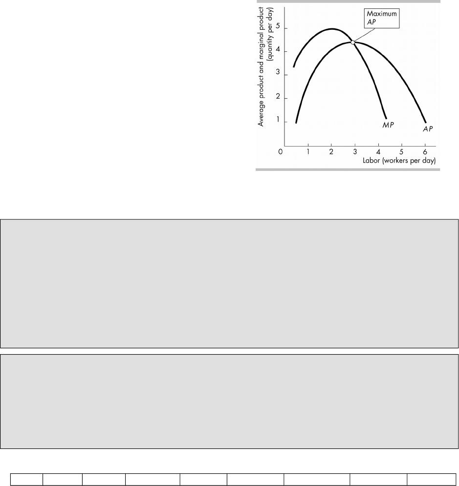
The marginal product curve shows the additional output generated by each
additional unit of labor. The marginal product of labor curve (MP) has an
upside-down U shape. Increasing marginal returns occurs when the marginal
Labor
Total
product
Marginal
product
Averag
e
product
0 0
10
1 10 10
20
2 30 15
6
3 36 12
product of an additional worker is greater than the marginal product of the previous
worker. At low levels of employment, increasing marginal returns is likely because
hiring an additional worker allows large gains from specialization. Eventually these
gains become small or nonexistent and diminishing marginal returns set in.
Diminishing marginal returns occur when the marginal product of an additional
worker is less than the marginal product of the previous worker. The law of
diminishing returns states that as a rm uses more of a variable factor of
production, with a given quantity of the xed factor of production, the marginal
product of the variable factor eventually
diminishes.
The average product curve shows the
average product that is generated by
labor at each level of labor. As the gure
shows, the average product of labor
curve (AP) has an upside-down U shape.
As the gure shows, the marginal product
curve and the average product curve are
related: when the marginal product of
labor exceeds the average product of
labor, the average product of labor
increases; when the marginal product of
labor is less than the average product of
labor, the average product of labor
decreases; and the marginal product of
labor equals the average product of labor when the average product of labor is at its
maximum.
The marginal pulls (but cannot not push) the average. Don’t let the students fall into
the trap of thinking that if the marginal measure rises (falls) with the level of an activity,
then the average measure must also rise (fall). This is a sloppy statement of the
relationship between marginal and average measures. Use the tried-and-true grade point
average (GPA) example used in the text. Explain that if a student’s GPA is a 3.5 and the
next marginal class grade is a C (2.0), followed by a B (3.0), this increasing marginal grade
will not be pushing their GPA up at all. Conceptually, the students should understand that
the marginal value can’t “push” the average measure higher when it is, itself, lower than
the average measure. The marginal measure must be higher (lower) than the average
value if the average value is to rise (fall) with the level of activity, thereby “pulling” the
average up (down).
Understanding marginal returns: Ask students to picture a typical fast food
restaurant. This is a “plant” and equipment with which they are familiar as customers if
not also as workers. Fixed inputs include the building and the equipment. Ask them to
imagine one worker trying to cook the food, take the orders and run the drive through. Add
a second worker and specialization can begin to occur, so the MP initially rises. But keep
adding workers and marginal product will inevitably fall. Diminishing returns is not the
same as negative returns; students might need help understanding that total product is
still rising, but at a decreasing rate.
III. Short-Run Cost
Fixed Variable Total Average Average Average Margin
Lab
or
Outp
ut
cost
(dollar
s)
cost
(dollars)
cost
(dollar
s)
xed
cost
(dollars)
variable
cost
(dollars)
total cost
(dollars)
al cost
(dollars
)
0 0 50 0 50
10.00
1 10 50 100 150 5.00 10.00 15.00
5.00
2 30 50 200 250 1.66 6.67 8.33
16.67
3 36 50 300 350 1.39 8.33 9.72
The table above continues the previous product schedule table and shows di!erent costs.
Total Cost
Total cost (TC) is the cost of all the factors of production a rm uses. Total -xed
cost (TFC) is the cost of the rm’s xed factors. Total variable cost (TVC) is the
cost of the rm’s variable factors. Total cost is the sum of total xed cost plus total
variable cost so TC = TFC + TVC.
Relation between TP and TVC. Make a graph of a TP curve on a transparency. Label the
x-axis labor and the y-axis output. Put some actual numbers on the labor axis (use 1, 2, 3,
4, and 5 labor units) and tell the students that the price of a unit of labor $10. Next,
change the label on the x-axis to TVC and ask the students to tell you the numbers to put
on the x-axis now that it measures TVC (the numbers will now be $10, $20, $30, $40 and
$50). Once the students are really clear about what you have done, pick up the
transparency, turn it over, and replace it on the display base with what was previously the
x-axis (TVC) running vertically. Point out that the students are now looking at a TVC curve.
Emphasize that all the product curves can be derived from the TP curve and all the cost
curves can be derived from the TVC curve.
Marginal Cost
Marginal cost (MC) is the increase in total cost that results from a one-unit
increase in output. The MC curve is U-shaped. Initially greater specialization makes
additional units cost less than those that have come before, but eventually
diminishing returns sets in and marginal costs rise.
Average Cost
Average -xed cost (AFC) is total xed cost per unit of output. The value of AFC
falls as output increases.
Average variable cost (AVC) is total variable costs per unit of output. At low levels
of output, AVC falls as output increases but at higher levels of output, AVC rises as
output increases.
Average total cost (ATC) is the total cost per unit of output. ATC = AFC + AVC. At
low levels of output, ATC falls as output increases but at higher levels of output, ATC
rises as output increases.
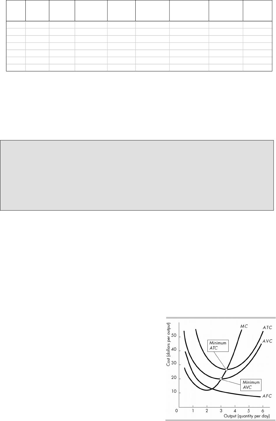
Marginal Cost and Average Cost
The gure illustrates typical MC, AFC, AVC,
and ATC curves. As the gure shows, the MC
curve, the AVC curve, and the ATC curve are
all U-shaped. There are other additional
important points about this gure:

The vertical distance between the AVC curve and the ATC curve is the AFC.
Because the AFC decreases as output increases, these curves become vertically
closer to each other as output increases.
The MC curve intersects the AVC curve and ATC curve at their minimums
Why the Average Total Cost Curve is U-shaped
The ATC curve combines the shapes of the AFC and AVC curves. The AFC curve
constantly falls as output expands, pulling down ATC curve. The AVC curve rst falls
but then rises because of diminishing returns. Eventually AVC curve starts to rise
more rapidly than the AFC falls, so at that point the ATC rises.
An Economics in the News case describes a new cost curve application insprired by
Walmart’s decision to increase use of self-checkout machines in its stores. The case derives
and analyzes the cost curves for both traditional clerks and for checkout assistants for
shoppers using self scan technologies.
Cost Curves and Product Curves
The shape of the AVC curve is determined by the shape of the AP curve. Over the
range of output for which the AP curve is rising, the AVC curve is falling and over the
range of output for which the AP curve is falling, the AVC curve is rising.
The shape of the MC curve is determined by the shape of the MP curve. Over the
range of output for which the MP curve is rising, the MC curve is falling and over the
range of output for which the MP curve is falling, the MC curve is rising.
Making Decisions Using the Relationships Between Productivity and Cost. Explain
to the students the usefulness of understanding the intuition behind the relationship
between productivity measures and cost measures. For example:
If a rm manager knows that average productivity of labor has been falling with the last
additional quantity of labor hired, then the manager knows that the average variable cost
(AVC) of production has necessarily been rising as the output from that additional labor
has increased.
If the manager knows that AVC is rising as output increases, then the manager also knows
that the marginal cost (MC) of the additional output has been higher than the AVC (which
has been pulling AVC up).
If the manager has sold the previous units of output at a small prot, the manager might
be faced with a time-sensitive contractual opportunity that arises within the same short
run time period. The manager might be asked to sell a little more output at the same
market price as the previous sales. The manager can quickly infer that the protability of
this potential new contract will not be as high because the marginal cost of producing the
extra output will be higher than the last units of output produced. The manager can infer
this result through productivity-cost relationships rather than knowing marginal costs
directly.
Firm managers must frequently make quick decisions with little information. If managers
have knowledge of a useful relationship between input measures (which are relatively easy
to get) and production cost measures (which are more di#cult to get—especially marginal
cost gures) they can use their understanding of this link to make inferences about how
production costs might behave when the rm’s output must change to accommodate
market changes.
Shifts in the Cost Curves
The cost curves shift with changes in technology or changes in prices of factors of
production.
An increase in technology that allows more output to be produced from the same
resources shifts the cost curves downward. If the technology requires more
capital, a xed input, then the average total cost curve shifts upward at low
levels of output and downward at higher levels of output.
A fall in the price of the xed factor shifts the AFC and ATC curves downward but
leaves the AVC and MC curves unchanged. A fall in the price of a variable factor
shifts the AVC, ATC, and MC curves downward but leaves the AFC curve unchanged.