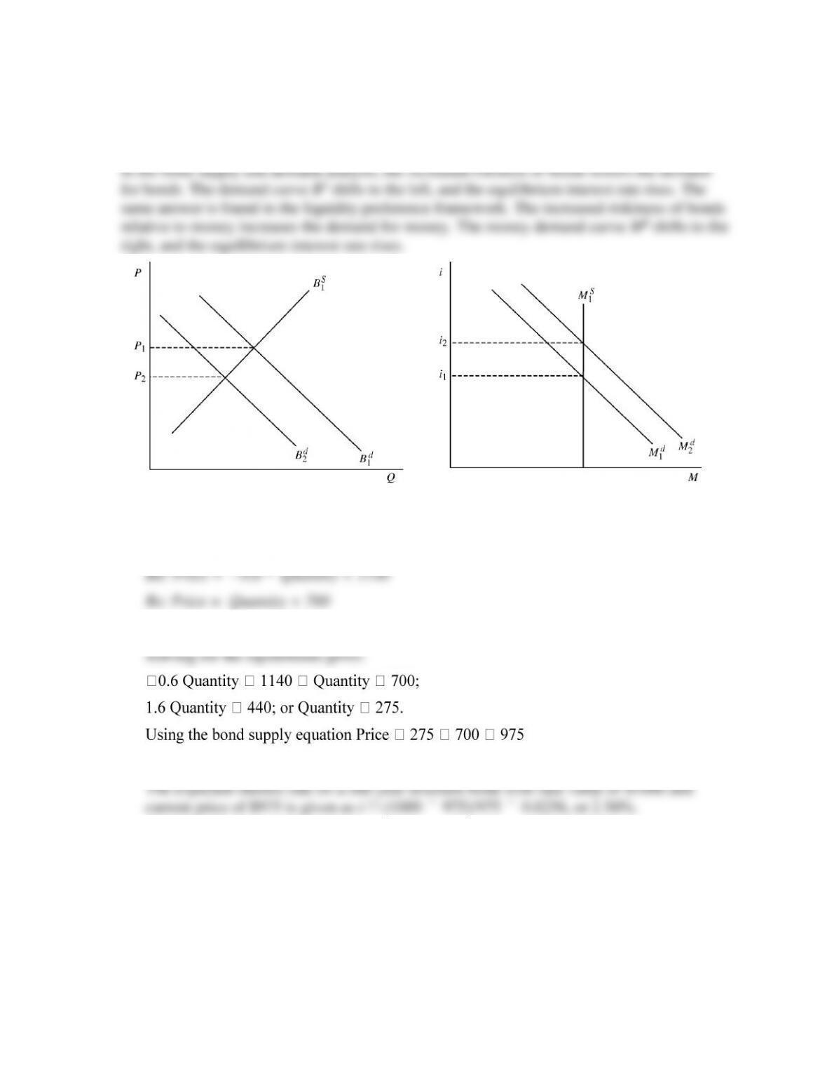
23. Using both the supply and demand for bonds and liquidity preference frameworks, show how
interest rates are affected when the riskiness of bonds rises. Are the results the same in the two
frameworks?
24. The demand curve and supply curve for one-year discount bonds with a face value of $1,000
are represented by the following equations:
a. What is the expected equilibrium price and quantity of bonds in this market?
b. Given your answer to part (a), what is the expected interest rate in this market?
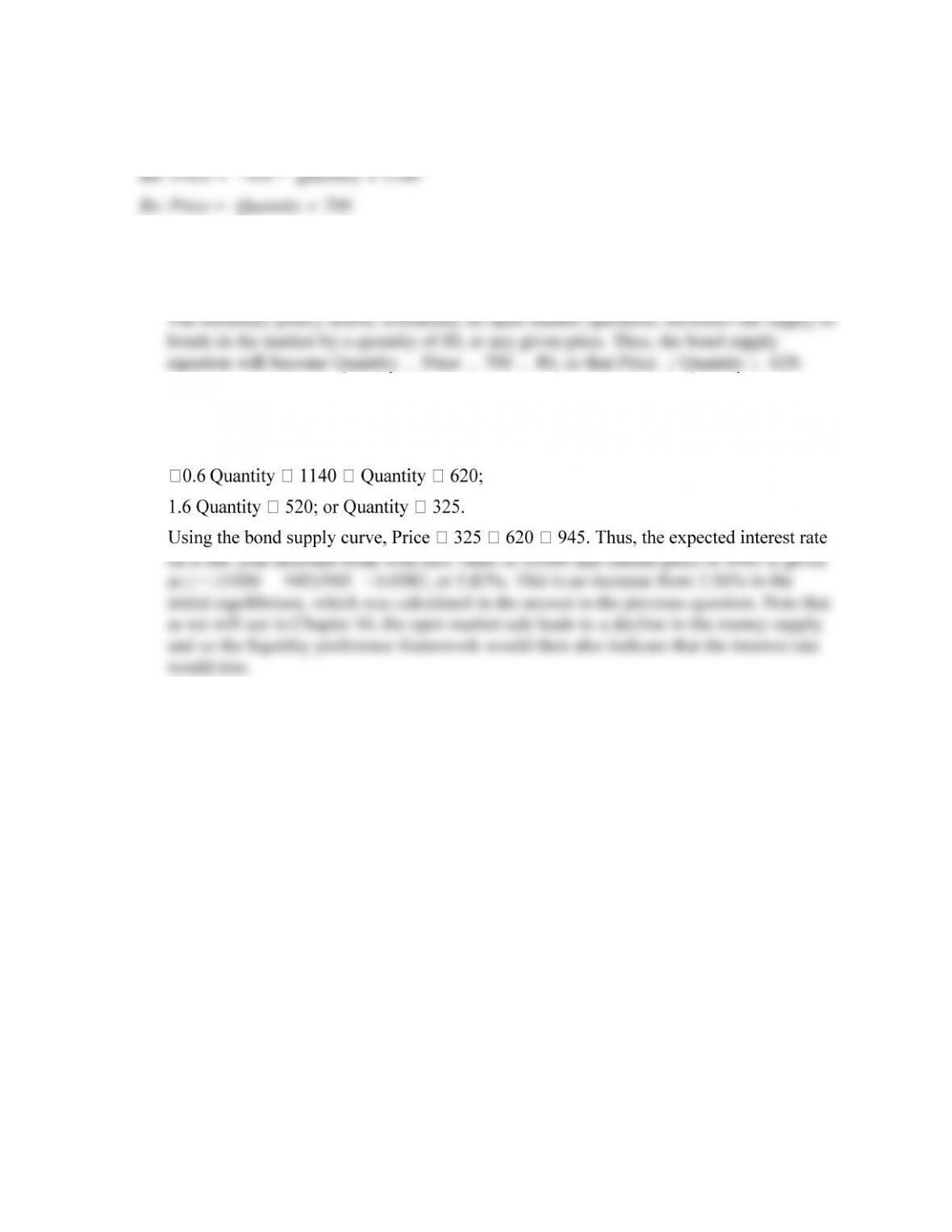
25. The demand curve and supply curve for one-year discount bonds with a face value of $1,000
are represented by the following equations
Suppose that, as a result of monetary policy actions, the Federal Reserve sells 80 bonds that
it holds. Assume that bond demand and money demand are held constant.
a. How does the Federal Reserve policy affect the bond supply equation?
b. Calculate the effect of the Federal Reserve’s action on the equilibrium interest rate in
this market.
As a result of the Federal Reserve action, the new equilibrium is given as:
ANSWERS TO DATA ANALYSIS PROBLEMS
1. Go to the St. Louis Federal Reserve FRED database, and find data on net worth of
households and non-profits (HNONWRQ027S) and the 10-year U.S. treasury bond (GS10).
For the net worth indicator, adjust the units setting to “Percent Change from Year Ago,” and
for the 10-year bond, adjust the frequency setting to “Quarterly.”
a. What is the percent change in net worth over the most recent year of data available? All
else being equal, what do you expect should happen to the price and yield on the 10-year
treasury bond? Why?
b. What is the change in yield on the 10-year treasury bond over the last year of data
available? Is this result consistent with your answer to part (a)? Briefly explain.
2. Go to the St. Louis Federal Reserve FRED database, and find data on the M1 money supply
the units setting to “Percent Change from Year Ago,” and for the 10-year treasury bond,
adjust the frequency setting to “Quarterly.” Download the data into a spreadsheet.
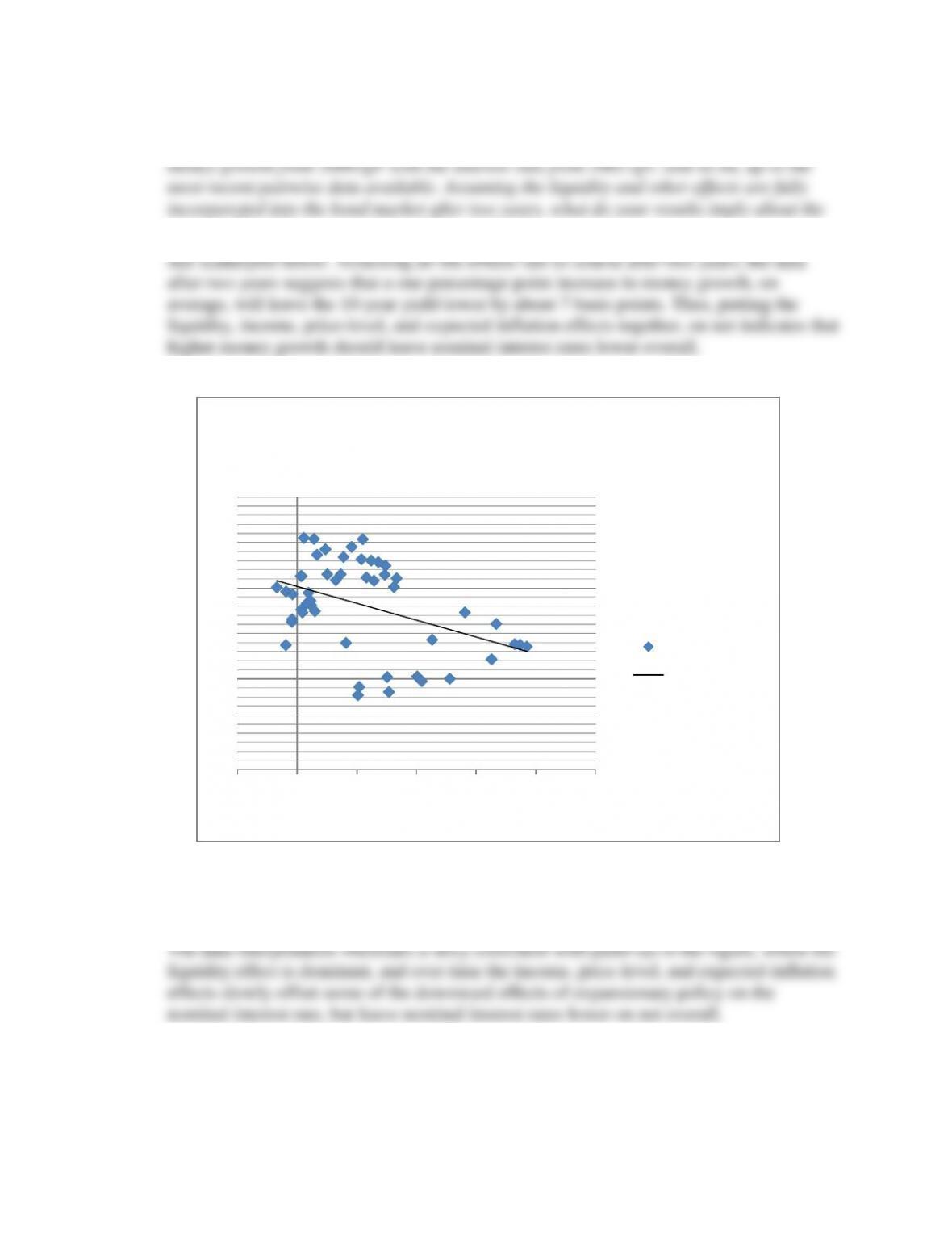
a. Create a scatter plot, with money growth on the horizontal axis and the 10-year treasury
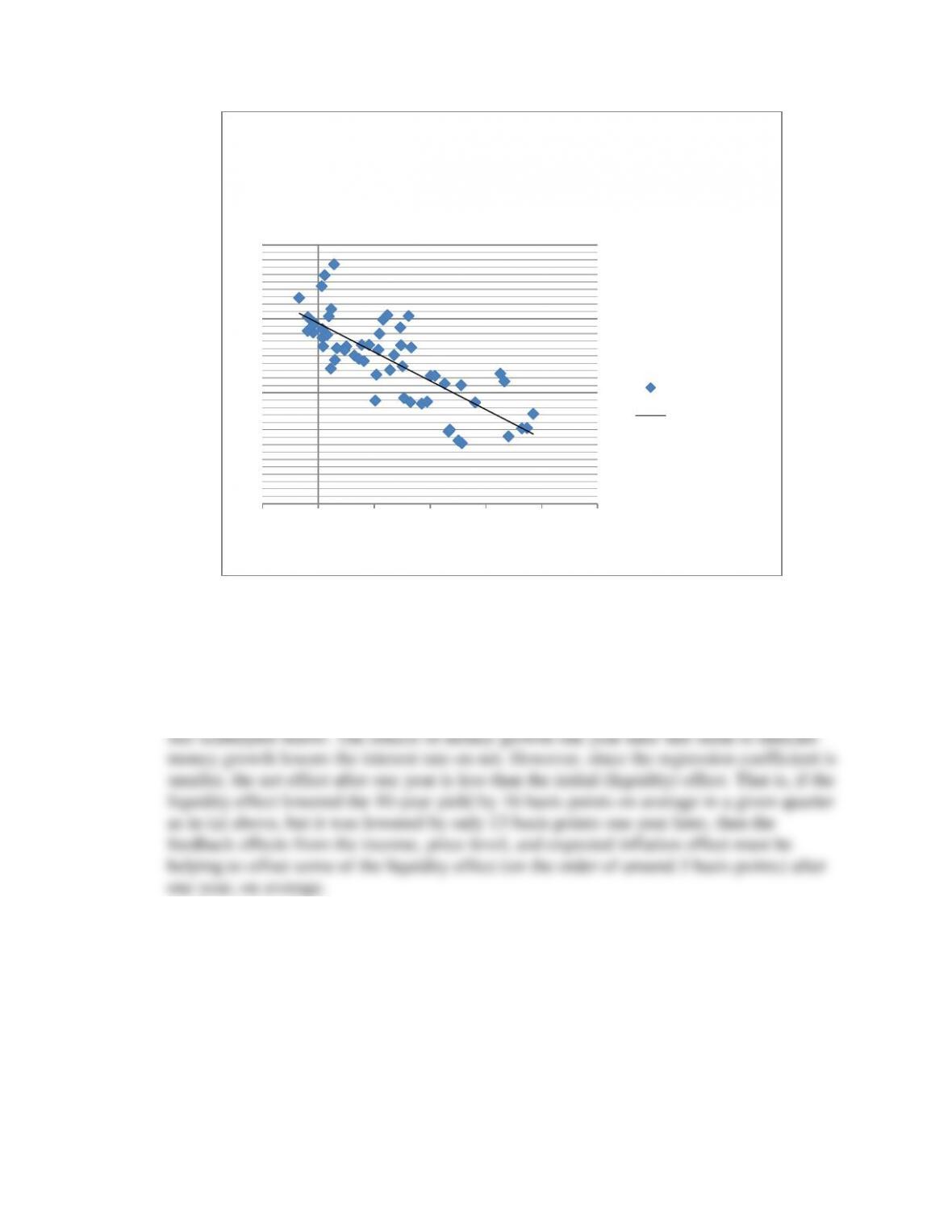
b. Repeat part (a), but this time compare the contemporaneous money growth rate with the
interest rate four quarters later. For example, create a scatter plot comparing money
growth from 2000:Q1 with the interest rate from 2001:Q1, and so on, up to the most
recent pairwise data available. Compare your results to those obtained in part (a), and
interpret the liquidity effect as it relates to the income, price-level, and expected-inflation
effects.
y = -0.1559x + 4.8835
R² = 0.602
0.00
1.00
2.00
3.00
4.00
5.00
6.00
7.00
-5.0 0.0 5.0 10.0 15.0 20.0 25.0
Interest Rate
Money Growth
Money Growth and
Contemporaneous 10-year rate
2000:Q1 to 2014:Q1
Series1
Linear (Series1)
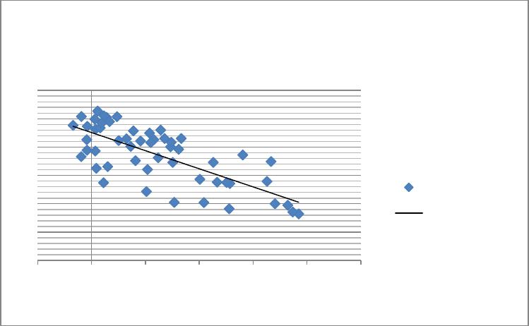
y = -0.1277x + 4.5096
R² = 0.5368
0.00
1.00
2.00
3.00
4.00
5.00
6.00
-5.0 0.0 5.0 10.0 15.0 20.0 25.0
Interest Rate
Money Growth
Money Growth and One Year Ahead
10-year rate 2000:Q1 to 2013:Q1
Series1
Linear (Series1)
c. Repeat part (a) again, except this time compare the contemporaneous money growth rate
with the interest rate eight quarters later. For example, create a scatter plot comparing
overall effect of money growth on interest rates?
d. Based on your answers to parts (a) through (c), how do the actual data on money growth
and interest rates compare to the three scenarios presented in Figure 11 of this chapter?
y = -0.0742x + 4.0325
R² = 0.1799
0.00
1.00
2.00
3.00
4.00
5.00
6.00
-5.0 0.0 5.0 10.0 15.0 20.0 25.0
Interest Rate
Money Growth
Money Growth and Two Year Ahead
10-year rate 2000:Q1 to 2012:Q1
Series1
Linear (Series1)