Chapter 19
ANSWERS TO QUESTIONS
1. How would you expect velocity to typically behave over the course of the business cycle?
2. If velocity and aggregate output are reasonably constant (as the classical economists
believed), what will happen to the price level when the money supply increases from $1
trillion to $4 trillion?
3. If credit cards were made illegal by congressional legislation, what would happen to
velocity? Explain your answer.
4. “If nominal GDP rises, velocity must rise.” Is this statement true, false, or uncertain?
Explain your answer.
5. Why would a central bank be concerned about persistent, long-term budget deficits?
6. “Persistent budget deficits always lead to higher inflation.” Is this statement true, false, or
uncertain? Explain your answer.
7. Suppose a new “payment technology” allows individuals to make payments using U.S.
8. Some payment technologies require infrastructure (e.g., merchants need to have access to
credit card swiping machines). In most developing countries, this infrastructure is either
nonexistent or very costly. Everything else being equal, would you expect the transaction
component of the demand for money to be greater or smaller in a developing country than in
a rich country?
9. What three motives for holding money did Keynes consider in his liquidity preference theory of
the demand for real money balances? On the basis of these motives, what variables did he
think determined the demand for money?
The three motives are: precautionary, speculative, and transactions motives. From these three
10. In many countries, people hold money as a cushion against unexpected needs arising from a
variety of potential scenarios (e.g., banking crises, natural disasters, health problems,
unemployment, etc.) that are not usually covered by insurance markets. Explain the effect of
such behavior on the precautionary component of the demand for money.
11. In Keynes’s analysis of the speculative demand for money, what will happen to money
demand if people suddenly decide that the normal level of the interest rate has fallen? Why?
12. Why is Keynes’s analysis of the speculative demand for money important to his view that
velocity will undergo substantial fluctuations and thus cannot be treated as constant?
13. According to the portfolio theories of money demand, what are the four factors that
determine money demand? What changes in these factors can increase the demand for
money?
The four factors determining money demand under portfolio theory are: interest rates
14. Explain how the following events will affect the demand for money according to the portfolio
theories of money demand:
a. The economy experiences a business cycle contraction.
b. Brokerage fees decline, making bond transactions cheaper.
c. The stock market crashes. (Hint: Consider both the increase in stock price volatility
following a market crash and the decrease in wealth of stockholders.)
15. Suppose a given country experienced low and stable inflation rates for quite some time, but
then inflation picked up and over the past decade has been relatively high and quite
unpredictable. Explain how this new inflationary environment would affect the demand for
money according to portfolio theories of money demand. What would happen if the
government decided to issue inflation-protected securities?
16. Consider the portfolio choice theory of money demand. How do you think the demand for
money would be affected during a hyperinflation (i.e., monthly inflation rates in excess of
50%)?
The demand for money would decrease, similar to problem 15 above, but much more
17. Both the portfolio choice and Keynes’s theories of the demand for money suggest that as the
relative expected return on money falls, demand for it will fall. Why does the portfolio choice
approach predict that money demand is affected by changes in interest rates? Why did
Keynes think that money demand is affected by changes in interest rates?
18. Why does the Keynesian view of the demand for money suggest that velocity is unpredictable?
19. What evidence is used to assess the stability of the money demand function? What does the
evidence suggest about the stability of money demand, and how has this conclusion affected
monetary policymaking?
20. Suppose that a plot of the values of M2 and nominal GDP for a given country over 40 years
shows that these two variables are very closely related. In particular, a plot of their ratio
(nominal GDP/M2) yields very stable and easy-to-predict values. On the basis of this
evidence, would you recommend that the monetary authorities of this country conduct
monetary policy by focusing mostly on the money supply rather than on setting interest
rates? Explain.
ANSWERS TO APPLIED PROBLEMS
21. Suppose the money supply M has been growing at 10% per year, and nominal GDP, PY, has
been growing at 20% per year. The data are as follows (in billions of dollars):
2015
2016
2017
M
100
110
12
PY
1,000
1,200
1,440
Calculate the velocity for each year. At what rate is the velocity growing?
Velocity is approximately 10 in 2015, 10.9 in 2016, and 11.9 in 2017. The rate of velocity
growth is approximately 9% per year.
22. Calculate what happens to nominal GDP if velocity remains constant at 5 and the money
supply increases from $200 billion to $300 billion.
23. What happens to nominal GDP if the money supply grows by 20% but velocity declines by
30%?
24. If velocity and aggregate output remain constant at 5 and $1,000 billion, respectively, what
happens to the price level if the money supply declines from $400 billion to $300 billion?
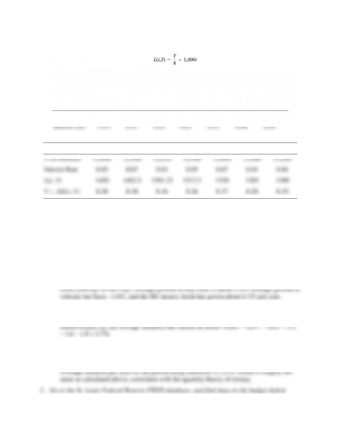
25. Suppose the liquidity preference function is given by
Use the money demand equation, along with the following table of values, to calculate the
velocity for each period.
Period
1
Period
2
Period
3
Period
4
Period
5
Period
6
Period
7
Y (in billions)
12,000
12,500
12,250
12,500
12,800
13,000
13,200
Interest rate
0.05
0.07
0.03
0.05
0.07
0.04
0.06
Period 1
Period 2
Period 3
Period 4
Period 5
Period 6
Period 7
Y (in billions)
12,000
12,500
12,250
12,500
12,800
13,000
13,200
Interest Rate
0.05
0.07
0.03
0.05
0.07
0.04
0.06
L(i, Y)
1450
1492.5
1501.25
1512.5
1530
1585
1590
V Y/L(i, Y)
8.28
8.38
8.16
8.26
8.37
8.20
8.30
ANSWERS TO DATA ANALYSIS PROBLEMS
1. Go to the St. Louis Federal Reserve FRED database, and find data on the M1 Money Stock
(M1SL), M1 Money Velocity (M1V), and Real GDP (GDPC1). Convert the M1SL data series
to “quarterly” using the frequency setting, and for all three series, use the “Percent Change
from Year Ago” setting for units.
a. Calculate the average percentage change in real GDP, the M1 money stock, and velocity
since 2000:Q1.
b. Based on your answer to part (a), calculate the average inflation rate since 2000 as
predicted by the quantity theory of money.
c. Next, find the data on the GDP deflator price index (GDPDEF), download the data using
the ‘Percent Change from Year Ago’ setting, and calculate the average inflation rate
since 2000:Q1. Comment on the value relative to your answer in part (b).
(FYFSD), the amount of federal debt held by the public (FYGFDPUN), and the amount of
federal debt held by the Federal Reserve (FDHBFRBN). Convert the two “debt held” series
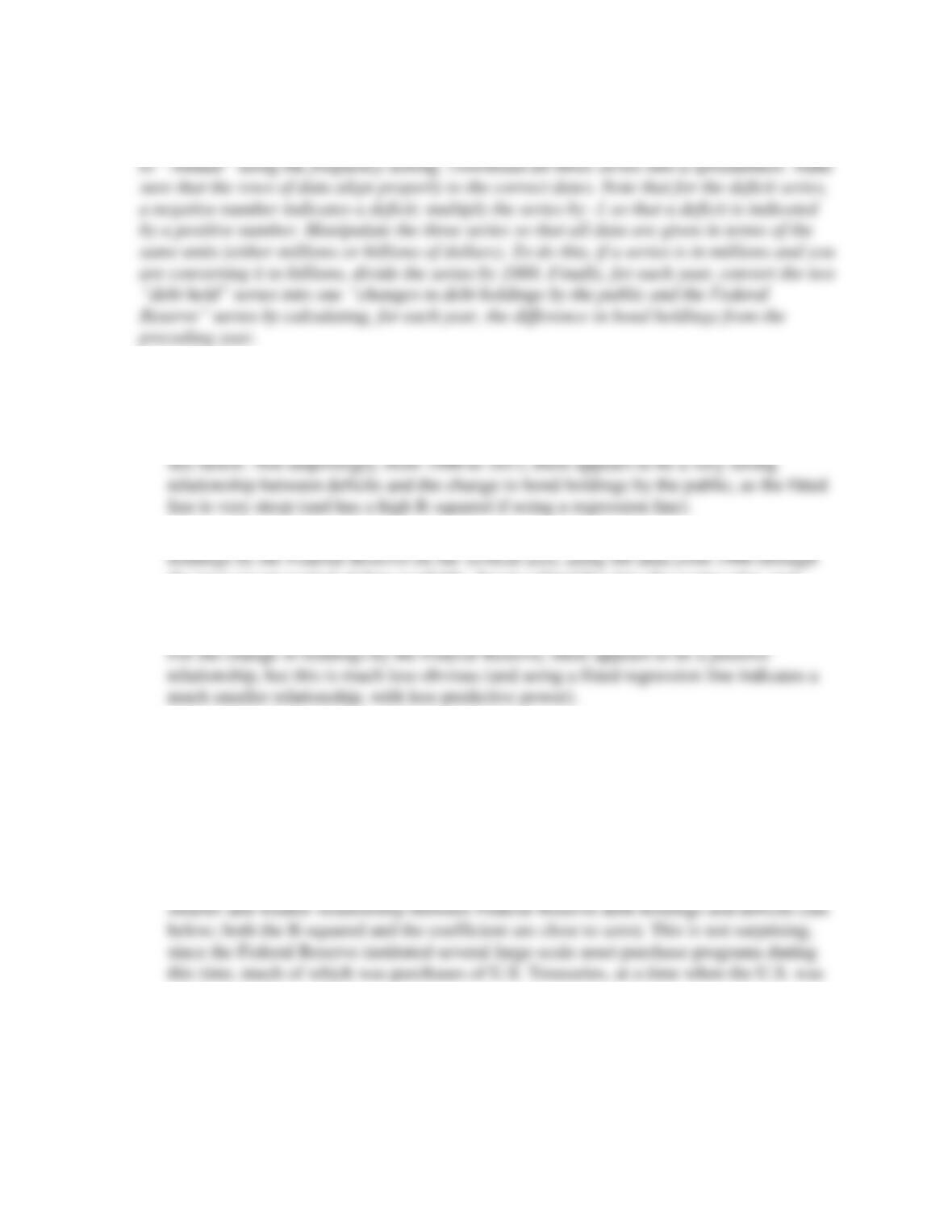
a. Create a scatter plot showing the deficit on the horizontal axis and the change in bond
holdings by the public on the vertical axis, using the data from 1980 through the most
recent period of data available. Insert a fitted line into the scatter plot, and comment on
the relationship between the deficit and the change in public bond holdings.
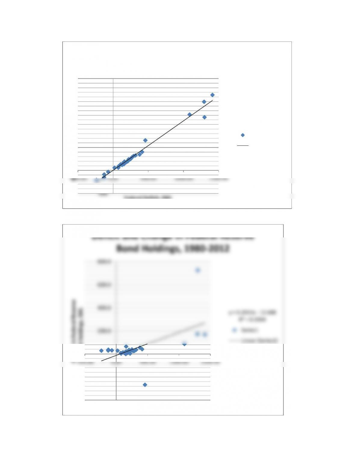
b. Create a scatter plot showing the deficit on the horizontal axis and the change in bond
the most recent period of data available. Insert a fitted line into the scatter plot, and
comment on the relationship between the deficit and the change in Federal Reserve bond
holdings.
c. Based on your results in parts (a) and (b), comment on how, if at all, the monetizing of
the debt is exhibited in the data. Do you think the relationship between the deficit and the
change in bond holdings of the Federal Reserve has changed since 2008? Why or why
not?
There appears to be some amount of debt monetization in the scatterplot data: in general,
as the deficits get larger, the change in bond holdings by the Fed gets larger, indicating
the central bank is facilitating higher deficits. However, this appears to be driven by the
large outlier deficits in the 2008 – 2012 period. Removing these data show a much
running very large deficits.
y = 1.0767x + 1.8904
R² = 0.9784
-500
0
500
1000
1500
2000
-500.00 0.00 500.00 1000.00 1500.00
Change in Public Bond Holdings, $Bil.
Federal Deficit, $Bil.
Deficit and Change in Public Bond
Holdings, 1980-2012
Series1
Linear (Series1)
-400.0
800.0
Deficit and Change in Federal Reserve
Bond Holdings, 1980-2012
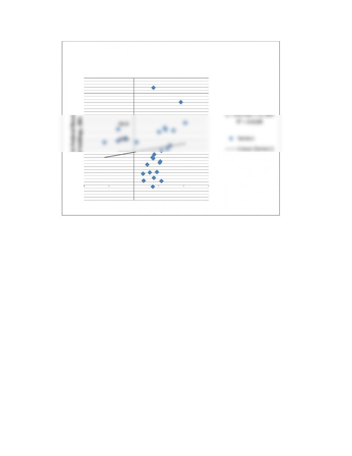
y = 0.0143x + 21.409
R² = 0.0185
-10.0
0.0
10.0
20.0
30.0
40.0
50.0
60.0
70.0
-400.00 -200.00 0.00 200.00 400.00 600.00
Change in Federal Reserve
Bond Holdings, $Bil.
Federal Deficit, $Bil.
Deficit and Change in Federal Reserve
Bond Holdings, 1980 – 2007
Series1
Linear (Series1)