CHAPTER 8
Quick Check
1. a. True.
b. False. After 1970 the relationship between inflation and unemployment broke down.
c. True
2. a. No. In the 1970s, we experienced high inflation and high unemployment. The
expectations-augmented Phillips curve is a relationship between inflation and
unemployment conditional on the natural rate and inflation expectations. Given inflation
b. This is not correct. The expectations-augmented Phillips curve implies that maintaining a
c. It does appear that workers resist reductions in nominal wages even when there is
3. a. Solve the equation where actual and expected inflation take the same value to
Now substitute for un. Then π_t
Objec t 1
c. The natural rate of unemployment is higher when the markup (m) is higher.
e. The list mentioned in the text includes the generosity of unemployment insurance
©2017 Pearson Education, Inc.
114
proportion of persons in young age groups; the proportion of employment in temporary
jobs; the unionization rate; the minimum wage; employment protection.
4. a. If the parameter is zero, then the expected rate of inflation is the constant
Objec t 2
. The
c. Choices will vary.
In this case
Objec t 3
in all periods since =0.
Initial unemployment is 0.05 or 5%. In period t, unemployment is reduced to 3%. If we
Objec t 4
Objec t 5
b. This does not make much sense. Every period actual inflation exceeds expected inflation
Objec t 6
c. This will put more weight on previous year’s inflation in forming the expectation of
inflation. In the periods from t+1 to t+5, a reasonable person might think last period’s
inflation (4 percentage points higher than
Objec t 7
) is a better predictor of actual inflation than
the fixed value
Objec t 8
.
d. The values will be: t+6: solving
0.1 2
e
t t t
up p= + –
and using
Objec t 10
= πt-1
t+6 ut+6 = .03 πt+6 =
Objec t 11
+.04 + 0.1 – (2 x .03) =
Objec t 12
+.04 + .04 =
Objec t 13
+.08
Objec t 14
Objec t 15
Objec t 16
Objec t 17
Objec t 18
Objec t 19
e. You can see that keeping unemployment below the natural rate leads to an ever
accelerating rate of inflation when =1. Hence the other name for the natural rate is the
f. If the unemployment rate is at the natural rate of unemployment (5%) and we assume that
©2017 Pearson Education, Inc.
115
Dig Deeper
6. a. This will move the model of expected inflation so that
π t = π t-1 – 2(ut – .05)= π t-1 + 2%=2%
b. π t = 0.5 π t + 0.5 π t-1 – 2(ut – .05)
7. a-c: You should be able to reproduce Figure 8-4 with one or two more years of data. It is not
likely that one or two years will lead to a different line or a different natural rate of
unemployment. You should see your line crossing the horizontal axis at about 6%.
Explore Further
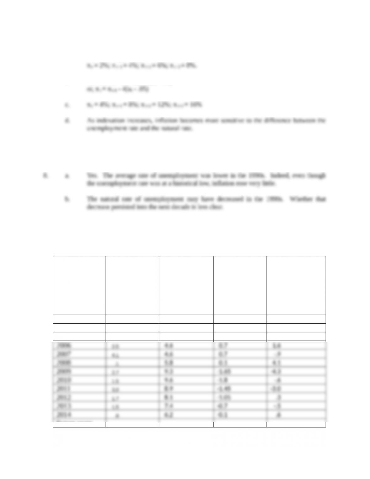
9. The filled in table will look like this
Year Inflation Unemployment Predicted
change in
inflation
Predicted change
in inflation minus
actual change in
inflation
2003 1.9 6.0 0 .5
2004 3.3 5.5 0.25 -1.2
2005 3.4 5.1 0.45 .4
Future years
©2017 Pearson Education, Inc.
116
a. There is no simple answer here. In some years 2003, 2005,2007, 2010, 2012, 2013, 2014
– the predicted change in inflation is within 1 percentage point of the actual change in
b. If we focus on the crisis years, 2009 and 2010, the model fits quite well in 2010. The high
level of unemployment in 2010 predicts a reduction in the inflation rate from 2009 to
c. Answers will vary.
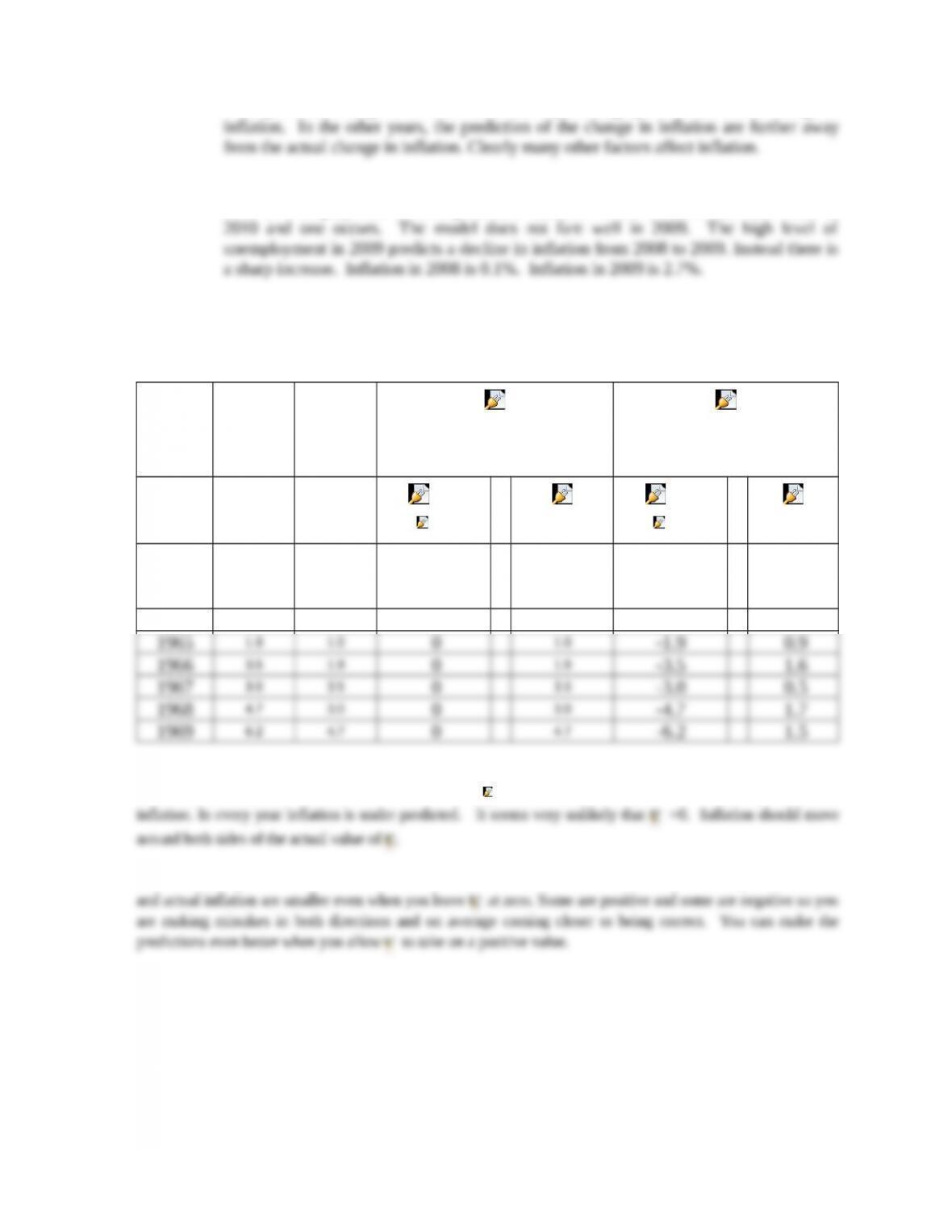
10. From the 1960’s
Year Actual
inflation
Lagged
actual
inflation
Objec t 20
Expected inflation under
different assumptions
Objec t 21
Difference: expected minus
actual inflation under
different assumptions
Year πtπt-1
Objec t 22
=0
and
Objec t 23
= 0
Objec t 24
=1.0
Objec t 25
=0
and
Objec t 26
= 0
Objec t 27
=1.0
1963 1.6 1.3 01.3
-1.6
0.3
1964 1.0 1.6 01.6 -1.0 -0.6
a. Zero is a poor choice for the both the value of and
Object 28
in the 1960s because it generates a poor prediction of
Object 29
Object 30
b. One is a better good choice for the value of in the 1960s because the differences between expected inflation
Object 31
Object 32
Fill in the values in the table below for inflation and expected inflation using the 1970s and 80s. You will have
the most success using a spreadsheet.
©2017 Pearson Education, Inc.
117
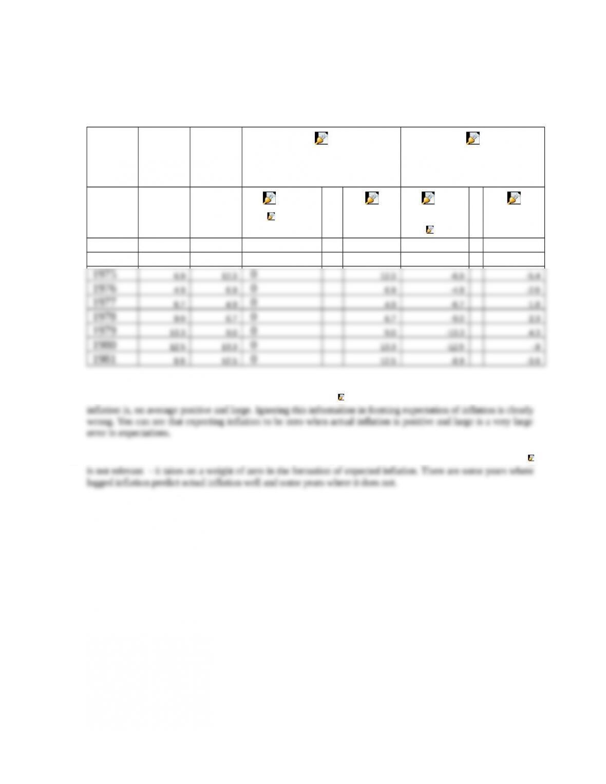
From the 1970’s and 1980’s:
Year Actual
inflation
Lagged
actual
inflation
Objec t 33
Expected inflation under
different assumptions
Objec t 34
Difference: expected minus
actual inflation under
different assumptions
Year πtπt-1
Objec t 35
=0
and
Objec t 36
= 0
Objec t 37
=1.0
Objec t 38
=
0
and
Objec t 39
= 0
Objec t 4 0
=1.0
1973 8.7 3.4 03.4 -8.7 5.3
1974 12.3 8.7 08.7 -12.3 3.6
c. Zero is now clearly a terrible choice for the value of and
Object 4 1
in the 1970s and early 1980s. It is clear that
d. One is a better choice for the value of in the 1970s and early 1980s. Once the value of is one, the value of
Object 4 2
e. The average level of inflation is clearly higher in the 1970s. Inflation also looks quite volatile in the 1970s –
there are large changes in inflation from year to year.
©2017 Pearson Education, Inc.
118