978-0133780581 Chapter 18 Lecture Note

Unlock access to all the studying documents.

View Full Document

Chapter 18. The Goods Market

in an Open Economy

I. MOTIVATING QUESTION

How is output determined in the short run in an open economy?

As in a closed economy, output in an open economy is determined by goods market equilibrium, the

condition that goods supply equals goods demand. In the open economy, however, goods demand

includes net exports.

II. WHY THE ANSWER MATTERS

The full treatment of short-run equilibrium in an open economy requires several steps. This chapter

integrates openness in the goods market into the model of goods market equilibrium. To consider the

goods market in isolation from financial markets, the chapter assumes that the interest rate is fixed and

treats the real exchange rate as a policy variable. Chapter 19 integrates openness in asset markets into the

determination of financial market equilibrium and then combines goods and financial market equilibrium

into an open-economy IS–LM model.

III. KEY TOOLS, CONCEPTS, AND ASSUMPTIONS

1. Tools and Concepts

i. The chapter introduces an open-economy model of goods market equilibrium by adding net

exports to the demand for domestic goods.

ii. A real depreciation will improve the trade balance when the proportional increase in relative

quantities (the sum of the proportional increase in exports and the proportional decrease in imports)

exceeds the proportional real depreciation. This condition is called the Marshall-Lerner condition. It is

derived in an appendix to the chapter.

iii. The J-curve describes the dynamics of trade balance adjustment after a real depreciation. Initially,

the trade balance falls, since the real depreciation tends to increase the relative value of imports. Over

time, however, consumers and firms start buying more home goods and fewer foreign goods (since real

depreciation makes home goods cheaper), and the trade balance improves.

18-82

2. Assumptions

The chapter considers the short-run goods market in isolation from financial markets, so it assumes that

the interest rate is fixed and that the real exchange rate is a policy variable. In keeping with the analysis

of Chapter 19, as well as the closed economy IS–LM analysis, a more precise way to state these

assumptions is that the home and foreign price levels are fixed and the nominal exchange rate is a policy

variable. Since the price levels are fixed, the nominal exchange rate determines the real exchange rate. In

addition, production is assumed to respond one-for–one to changes in demand without changes in price

(the AS curve is horizontal at the initial price), so demand determines output.

18-83

IV. SUMMARY OF THE MATERIAL

1. The IS Relation in the Open Economy

When the economy is open to trade in goods, it becomes important to distinguish the domestic demand

for goods, given by C+I+G, from the demand for domestic goods, denoted by Z and given by

Z=C+I+G-IM/+X.

(18.1)

As in Chapter 5, the domestic demand for goods is C(Y-T)+I(Y,r)+G. Real exports (X) and real imports

(IM) are given by the following expressions.

IM=IM(Y,). (18.2)

+ +

X=X(Y*,). (18.3)

+ –

Exports increase when foreign income (Y*) increases, since foreigners have more to spend, and when

there is a real depreciation (an decrease in ), since home goods become less expensive relative to foreign

goods. Imports increase when domestic income increases, since home residents have more to spend, and

when there is a real appreciation, since foreign goods become less expensive relative to domestic goods.

Figure 18-1 displays graphically the effect of introducing net exports into the model of goods market

equilibrium. The domestic demand for goods is denoted DD. To derive the demand for domestic goods,

first shift the DD curve down by the value of imports (IM/). The new curve, denoted AA, is flatter than

DD, because the value of imports increases with income. Now add exports to the AA curve to arrive at

the demand for domestic goods (ZZ). Note that exports are independent of income, so the vertical

distance between ZZ and AA is constant and the two curves have the same slope. The gap between the

curves DD and ZZ is the trade balance (sometimes called net exports (NX)), depicted in the lower panels

(c & d) in Figure 18-1. Since the value of imports increases with income, the trade balance decreases

with income. Note that Figure 18-1 assumes that the real exchange rate is fixed.

18-84

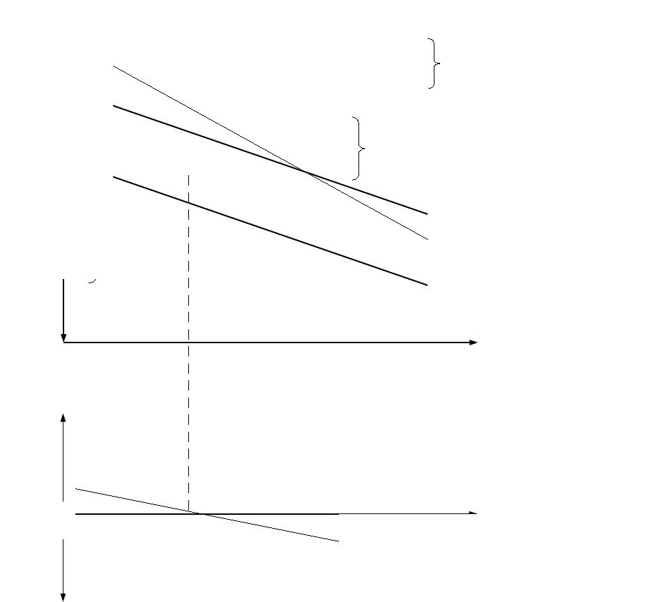
Figure 18-1c and d: The Demand for Domestic Goods and the Trade Balance (NX)

2. Equilibrium Output and the Trade Balance

Equilibrium in the goods market requires that the demand for domestic goods equals the production of

domestic goods, namely that Y=Z. Substituting equations (18.2) and (13.3) into the demand for domestic

goods results in a new IS relation:

Y=C(Y-T)+I(Y,r)+G-IM(Y,)/ +X(Y*,).

(18.4)

Note that real imports, which have units of foreign goods, are multiplied by the real exchange rate to

convert them into units of domestic goods.

Trade Balance, NX

0Income, Y

Domestic Demand (DD)

Demand for Domestic Goods (ZZ)

Income, Y

18-85

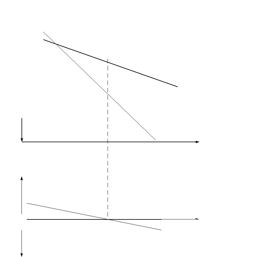
Since this chapter concentrates on the short run, it assumes that production responds one-for-one to

changes in demand (without changes in price). Graphically, equilibrium is determined by the intersection

of the ZZ curve and the 45°- line (Figure 18.2). In general, equilibrium does not require balanced trade.

Figure 18-2 depicts an equilibrium condition with a trade deficit.

Figure 18-2: Equilibrium Output and the Trade Balance (NX)

Trade Balance, NX

0Income, Y

45º

Demand for Domestic Goods (ZZ)

Income, Y

18-86

3. Increases in Demand – Domestic or Foreign

When domestic demand increases (e.g., G increases, T decreases, or consumer confidence increases), the

ZZ curve shifts up, so output increases and the trade balance falls. When foreign demand (Y*) increases,

the ZZ and NX curves shift up by the same amount. Output and the trade balance increase. The increase

in imports that arises from the increase in home output does not entirely offset the positive effect on

exports from the increase in foreign demand.

Note that increases in domestic demand have a smaller effect on output in the open economy than in the

closed economy, because some of the increased income “leaks” out of the domestic economy through

spending on imports. In other words, the multiplier is smaller in an open economy. A box in the text

carries this analysis further and notes that smaller countries are likely to have larger marginal propensities

to import out of income. As a result, fiscal policy will have a smaller effect on output in a smaller

economy, but a greater effect on the trade balance.

The relationship between foreign and domestic output suggests that policy coordination can be important

when industrial countries as a group are operating below normal levels of output. Governments typically

do not like to run trade deficits, because deficits require borrowing from the rest of the world. In the

absence of coordinated action, an expansionary policy by an individual country in the midst of a

worldwide recession will likely generate a trade deficit (or at least worsen the trade balance), because the

increase in income will increase imports. Coordinated expansions will tend to have less effect on trade

balances in individual countries, because imports will increase substantially throughout the world. On the

other hand, coordinated expansions may be difficult to arrange. Countries that have budget deficits may

be unwilling to consider expansionary fiscal policy. In addition, once an agreement has been negotiated,

each country has an incentive to renege, thereby hoping to benefit from expansions abroad and to improve

its trade balance.

4. Depreciation, the Trade Balance, and Output

The trade balance (NX) is given by

NX=X(Y*,) – IM(Y,)/.

A real depreciation has two effects: a quantity effect (an increase in exports and a reduction in imports),

which tends to increase the trade balance, and a price effect (an increase in the relative price of imports),

which tends to reduce the trade balance. The net effect will be positive if the quantity effect is greater

than the price effect, a condition known as the Marshall-Lerner condition (derived in an appendix). If so,

a real depreciation will improve the trade balance and increase output. With some qualifications, the

Marshall-Lerner condition is usually satisfied in practice, and the text assumes that a real depreciation

will improve the trade balance.

If the government can affect the real exchange rate through policy, then it can use two policy instruments

(fiscal policy and the real exchange rate) to achieve two policy targets (output and the trade balance). For

18-87

example, suppose a country in recession has a trade deficit, and policymakers want to achieve the natural

level of output and balanced trade. Expansionary fiscal policy will increase output, but will also worsen

the trade deficit. A real depreciation will increase output and improve the trade deficit, but there is no

guarantee that it can achieve the output target under balanced trade. To achieve both targets,

policymakers need a policy mix: in this case, a real depreciation sufficient to balance trade at the target

output level and the fiscal policy required to ensure that the economy achieves the target output level. If

output is higher than desired after the real depreciation, policymakers should use contractionary fiscal

policy; if output is lower than desired, policymakers should use expansionary fiscal policy. The text

includes a table that summarizes other policy mixes under alternative initial conditions for output and the

trade balance.

5. Looking at Dynamics: the J-Curve

The effects of a real depreciation have a dynamic dimension. The price effect happens immediately, but

the quantity effect takes time. As a result, the trade balance tends to worsen immediately after a real

depreciation, but to improve over time. In other words, it takes some time for the Marshall-Lerner

condition to be satisfied. This adjustment process of the trade balance—a temporary fall followed by a

gradual improvement—is called the J-curve. Econometric evidence suggests that in rich countries, the

trade balance improves between six months and a year after a real depreciation.

6. Saving, Investment, and the Current Account Balance

The national income identity (equation (18.1)) can be expressed as

NX = Y–C–I–G = (S–I) + (T–G),

where private saving (S) is given by S = Y–C–T. The first equality in equation says that the trade balance

equals income minus spending. The second equality of equation says that the trade balance is the excess

of private saving over investment plus the government budget surplus. Ignoring the distinction between

the current account and the trade balance, a trade surplus implies that a country is lending to the rest of

the world. The funds for this lending are derived from the two sources on the RHS of equation.

Since saving and investment are endogenous, this formulation can be a misleading guide for policy

analysis. For example, since the real exchange rate does not appear in this equation one might conclude

that a real depreciation has no effect on the trade balance. In fact, a real depreciation affects output, and

therefore affects saving and investment. If the Marshall-Lerner condition is satisfied, a real depreciation

will increase saving more than it increases investment, and improve the trade balance.

A box in the text examines the increase in the current account deficits of Euro periphery countries such as

Spain and Portugal. These current account deficits increased to high levels by 2008, the year the financial

crisis emerged. The higher borrowing costs for these nations forced them to reduce their current account

deficits as foreign borrowing proved too costly. However, given that exchanges could not adjust the

impact was to decrease output and imports. This adjustment is known as import compression and resulted

in an approximate 25% decline in both categories since 2008.

18-88

V. PEDAGOGY

The relationship between saving and investment in an open economy is presented at the end of the

chapter. There are two arguments for placing it at the beginning. First, the derivation of equation

presented in section 6 illustrates that the trade balance is the difference between income and spending.

Second, by discussing this equation before the policy experiments, instructors can include the effects on

saving and investment in the discussion of fiscal and exchange rate policy. This approach will reinforce

the notion that saving and investment are endogenous and that the government surplus is not the only

determinant of the trade balance. To illustrate the latter point, note that the U.S. federal budget deficit

declined over the 1990s, but the trade deficit reached record levels.

18-89