Chapter 14. Financial Markets and Expectations
I. MOTIVATING QUESTION
How can consumers and firms compare present and future economic
opportunities?
Future economic opportunities (payments received or made) can be expressed in terms of the present by
using a discount factor, which acts like a price. The sum of a sequence of payments, each priced at the
appropriate discount factor, is called the present discounted value of the sequence. In practice, future
variables are not known, so one calculates the expected present discounted value, which is the present
value of the expected sequence of payments.
II. WHY THE ANSWER MATTERS
Economic agents have foresight, so beliefs about the future can affect the present. This chapter describes
the basic tools by which consumers and firms can price future economic events (payments made or
received). In so doing, this chapter lays the groundwork for a look at consumption and investment
decisions when agents are forward-looking, a discussion of asset markets, and an integration of
expectations into IS-LM analysis. These topics are the subject of the next two chapters. Two important
applications—the determination of stock and bond prices—are analyzed in this chapter. The concept of
asset bubbles is also introduced.
III. KEY TOOLS, CONCEPTS, AND ASSUMPTIONS
1. Tools and Concepts
i. The expected present discounted value of a sequence of payments is the value today (i.e., in
current nominal or real units) of the expected sequence of payments.
ii. The relationship between yield and maturity is introduced via the yield curve.
iii. The concept of asset bubbles and the impact on the economy is introduced.
IV. SUMMARY OF THE MATERIAL
1. Expected Present Discounted Values
An investment of $1 today would grow to $[(1+it)(1+it+1)…(1+it+n-1)] in n years, if the investment
proceeds were reinvested. Thus, to accumulate $1 in n years, one would have to invest an amount
©2017 Pearson Education, Inc. Publishing as Prentice Hall
14-66
$Vt=1/[(1+it)(1+it+1)…(1+it+n-1)].
The required investment today is called the present value of $1 received in n years. This observation can
be used to calculate the present value of any stream of future payments. Typically, however, neither
future payments nor interest rates are known with certainty, so present value calculations must rely on the
expected values of future payments and short-run interest rates. Sequences with constant interest rates
and constant payments—over a fixed or infinite horizon—represent special cases. When future payments
are expressed in real terms, they are appropriately discounted using current and expected future real
interest rates. In most cases we shorten the name of the concept to present valueand the process of
computing a present value is known as discounting.
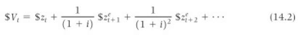
When we focus on a sequence of payments we can expand this formula to;
Variations depend on whether the cash flows are constant or vary from period to period. This formula, and
other formulations of this formula, has numerous applications including computing mortgage payments or
car payments and making investment decisions using the net present value (NPV) method.
2. Bond Prices and Bond Yields
Bonds differ based on maturity and risk. Maturity is the length of time over which the bond promises to
make payments while risk refers to the likelihood of default. Bond prices vary according to both factors.
Bondholders earn a yield, or yield to maturity (YTM), which is the interest rate earned if purchased at the
market price and held until the bond matures. A bond’s price is the present value of all expected future
cash flows.Note that you can use the present value formula (14.2) to compute the value of a bond. The
bond payments and maturity value are the cash flows and the discount rate (i) is the market rate on similar
risk bonds.
Bond yields differ based on time to maturity. This relationship between time to maturity and yield is
referred to as the term structure of interest rate. The graphical expression of the term structure of interest
rates is known as the yield curve (see Figure 14-2). A bond’s price is the present value of all expected
future cash flows when the YTM is used as a discount rate. For this reason, it is a simple process of
computing YTMs if you have a current price. These rates can then be plotted to graph the yield curve. Of
course, we invoke ceteris paribus and use the same issuer to compute the yield curve. U.S. Treasury
securities are used in practice. Yields curves are typically upward sloping (normal) but they can be
downward sloping (inverted). In general, the yield can provide us with information about investor
expectations with regard to interest rates.
©2017 Pearson Education, Inc. Publishing as Prentice Hall
14-67
3. The Stock Market and Movements in Stock Prices
Firms, unlike the government, receive some of their financing from sources other than debt. Firms can
either earn money (internal finance) or sell shares of ownership known as stock (external finance).
Investors buy stocks hoping the fractional ownership will increase in value as the firm prospers and stocks
also pay cash distributions known as dividends.
Stock prices, much like bonds, should be equal to the present value of all future cash flows. The future
cash flows are dividends and a future selling price. The rate of return used to discount the cash flows can
vary depending on risk and also market rates of interest. So, in the real world, a stock’s value is dependent
on future cash flows and the discount rate. Both of those factors can and do change periodically causing
constant revaluation of a stock.
One valuation model assumes infinite holding periods and values the stock as simply the present value of
all future dividends and it assumes the stock is not sold.
4. Risk, Bubbles, Fads, and Asset Prices
Stock prices change in value according to changes in expected future returns and perceived risk. And,
given the risk premium (x) is not constant, valuation shifts accordingly. For this reason, stock prices are
reasonably volatile.
At times stock prices deviate from their fundamental value which is defined as the present value of all
future dividends. Sometimes investors are willing to pay more for a stock than it is truly worth based on
their expectations. In other words, a stock price may increase above its fundamental value simply because
investors expect it to go up. This type of price movement is dubbed rational speculative bubbles.
At other times investors respond to fads and bid stock prices higher. Fads can occur in many markets,
including housing and stocks. See the Focus box on page 385 for a classic case of an asset bubble in the
tulip bulb market in the 1600s.
V. PEDAGOGY
This chapter marries two issues: the distinction between real and nominal interest rates and the calculation
of expected present discounted values. Depending upon the focus of the course, instructors could make
the distinction between real and nominal interest rates and ignore the mathematics of present values. It is
also possible to discuss the effects of expected future policies (Chapter 16) without a full presentation of
present value. In this context, instructors could describe informally how consumption and investment
decisions (examined in Chapter 15) depend upon current and expected future income and interest rates.
VI. EXTENSIONS
The presentation of present value in the text can be applied to numerous concepts in the students’ personal
lives. Taking a few minutes to go over some of these applications can help them understand present
values better. Alternatively, instructors might want to explain informally that attitudes toward risk affect
©2017 Pearson Education, Inc. Publishing as Prentice Hall
14-68
the value of risky payment streams. In particular, distaste for risk tends to reduce the value of risky
payments relative to the value of riskless ones.
VII. OBSERVATIONS
1. Discount Factors as Prices
The discount factor dt=1/(1+it) is a relative price that converts future dollars into present dollars. It plays
the same role in present value calculations that market prices do in GDP. Likewise, the real discount
factor, 1/(1+rt), converts future goods into current goods.
2. Indexed Bonds
The text constructs a series for the U.S. real interest rate by using OECD forecasts of inflation.
Historically, economists have been unable to observe U.S. real interest rates directly. However, in 1997,
the United States began offering Treasury bonds with payments indexed to the CPI inflation rate. The
prices of these bonds allow economists to construct a direct measure of the U.S. real interest rate. A
number of other countries also offer bonds with payments indexed to inflation.
©2017 Pearson Education, Inc. Publishing as Prentice Hall
14-69