978-0133780581 Chapter 11 Lecture Note

Unlock access to all the studying documents.

View Full Document

Chapter 11. Saving, Capital

Accumulation, and Output

I. MOTIVATING QUESTION

Does the saving rate affect growth?

If the production function exhibits decreasing returns to capital, an increase in the saving rate can only

affect the growth rate temporarily. In the long run, saving does not affect growth, but does affect the level

of output per worker.

II. WHY THE ANSWER MATTERS

Many macroeconomists are concerned about the low U.S. saving rate (relative to other OECD economies)

and the large scale of U.S. borrowing abroad. Changes in the structure of the Social Security system may

also have implications for saving and capital accumulation. This chapter clarifies the relationship

between saving, output per person, and growth, and discusses the likely effects of increasing the saving

rate.

III. KEY TOOLS, CONCEPTS, AND ASSUMPTIONS

1. Tools and Concepts

i. The chapter develops the Solowmodel of growth for the case of no technological change and no

population growth.

ii. The golden-rulelevel of capital per worker is the value of capital per worker that maximizes

steady-state consumption per worker.

iii. The Cobb-Douglas production function is described in an appendix.

2. Assumptions

This chapter assumes a closed economy, a fixed labor force, and a fixed level of technology.

IV. SUMMARY OF THE MATERIAL

1. Interactions between Output and Capital

There are two relations between output and capital;

1. The amount of capital determines the amount of output produced.

11-52

2. The amount of output determines savings which in turn determines capital accumulation over time.

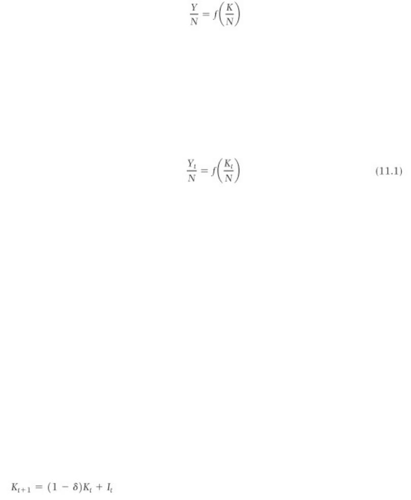
To save notation, write the aggregate production function of the previous chapter, Y/N=F(K/N,1), as

Now make the following assumptions.

i. There is no technological change.

ii. Population, the labor force participation rate, and the natural rate of unemployment are all

constant. Thus, N, interpreted as the natural level of employment, is also constant. We have also

introduced time indexes (t) for output and capital. The production function can now be written as;

Now we can see that higher capital per worker leads to higher output per worker.

Output and Investment

To derive the relationship between output and investment we make three assumptions.

i. The economy is closed.Investment, I, is equal to private saving, S, and public saving, T – G.

I = S + (T – G)

ii. Public saving (T – G) is equal to zero. This assumption allows us to focus on private saving.So,

Investment is equal to private saving, or I = S.

iii. Private saving is proportional to income;

S=sY.

Now we can combine these relations and see the following relationship between investment and output.

It =sYt

Investment and Capital Accumulation

Capital depreciates at rate,. Thus, the change in the capital stock over time is

Investment creates new capital, but the existing capital stock depreciates. Any change in capital at the end

of the year is the net effect of new investment and depreciation of existing capital.

2. The Implications of Alternative Saving Rates

The equations above together imply

11-53

((Kt+1/N)-(Kt/N)) =sf(Kt/N)– δ(Kt/N) (11.3)

Capital per worker increases to the extent that total saving per worker exceeds depreciation of the existing

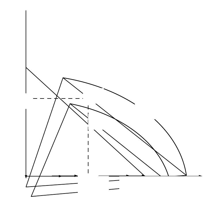
capital stock per worker. Figure 11-2 plots the separate components of equation (11.3).

Figure 11-2: Capital and Output Dynamics

The dynamics of adjustment are indicated by the arrows on the horizontal axis of Figure 11-2. To the left

of point A, saving per worker (sf(K/N)) exceeds depreciation of the existing stock (K/N), so the capital

stock per worker (K/N) rises. To the right of point A, K/N falls, since depreciation exceeds saving. These

dynamics imply that in the in the long run, the economy will arrive at point A. Once the economy reaches

this point, K/N and Y/N will remain constant. For this reason, the state of affairs represented by point A is

called a steady state for the economy. From equation (11.3), the steady-state value of K/N is determined

sf(K*/N)= (K*/N) (11.4)

K/N

f(K/N)

sf(K/N)

(Y*/N)

(K*/N) Capital per Worker, K/N

Output per Worker, Y/N

11-54

Point B indicates steady-state output per worker, which is given by

Y*/N=f(K*/N). (11.5)

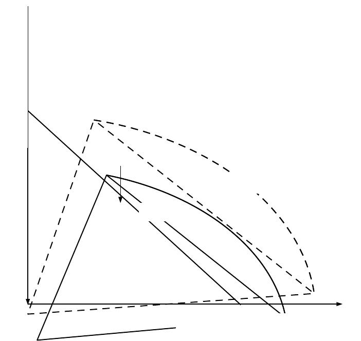
Now consider an increase in the saving rate. In Figure 11-3, an increase in the saving rate from s to s‘

shifts the sf(Kt/N) curve upward in proportion to the change in the saving rate. The new steady-state

equilibrium is given by point B. At this point, the steady-state growth rate (which is zero) is the same as

the original steady-state growth rate. Capital per worker, however, is higher at point B, so output per

worker is higher as well. These results imply that an increase in the saving rate will increase the growth

rate temporarily, since output per worker must increase to reach the new steady state, but not in the long

run.

Figure 11-3: The Effects of Different Saving Rates

What is the optimal saving rate? A very low saving rate will result in very low steady-state output and

consumption per worker. A very high saving rate will waste resources on depreciation, since extra units

of capital per worker produce very little extra output per worker when the capital stock is high.

Somewhere in between is a saving rate that maximizes steady-state consumption per worker. This rate is

called the golden rule saving rate, which produces the golden rule capital stock.

Empirically, it appears that the U.S. saving rate is below the golden rule rate, so it seems likely that an

increase in the saving rate would increase the consumption of future generations. On the other hand, an

K/N

sf(K/N)

sf(K/N)

Capital per Worker, K/N

Output per Worker, Y/N

11-55

increase in the saving rate would reduce the level of consumption for some time, until the increased

output (generated by the higher capital stock) compensated for the reduction in the proportion of output

consumed.

With these results in mind, a box in the text considers the effects of two proposals to reform the Social

Security System. A shift from a pay-as-you-go to a fully funded Social Security system could lead to a

higher capital stock in the long run, since Social Security contributions are invested and not simply

redistributed as in a pay-as-you-go system. This result, however, depends on how the transitional costs

are financed. If additional debt is issued to finance benefit payments during the transition, there will be

no effect on national saving, as the newly-issued debt will offset the additional saving from a fully funded

system. On the other hand, if additional taxes are raised or benefits are cut during the transition, then

some generation(s) will bear an extra burden beyond financing the retirement of the previous generation.

These considerations seem to imply that a shift to a fully funded system would have to be gradual, to

prevent the costs from falling too heavily on one generation. Similar issues would arise if workers were

allowed to divert a portion of Social Security payroll taxes into private retirement accounts. Either the

lost revenue would be borrowed, which would nullify the extra saving from the private accounts, or

financed by additional taxes and benefit cuts, which would imply that some generation(s) would bear an

additional burden.

3. Getting a Sense of Magnitudes

A Cobb-Douglas production function with equal shares of labor and capital implies that the capital

accumulation equation can be written

(Kt+1/N- Kt/N)=s(Kt/N)1/2–Kt/N.

In steady state,

s/=(K*/N)1/2=Y*/N.

In this case, if the saving rate doubles, so does long-run output per worker. How fast does the economy

adjust? Suppose that s increases from 0.1 to 0.2, that the depreciation rate equals 0.1, and that initially

K/N=1. Using the dynamic equation (11.3), one can show that adjustment to the new steady state is only

63% complete after 20 years.

With the same Cobb-Douglas production function, consumption per worker can be written

C*/N=(1-s)Y*/N=(1-s)s/,

which is maximized when s=1/2. Recall that the U.S. saving rate since 1950 has only been about 17%, so

if this model provides even a gross approximation of the U.S. economy, the U.S. saving rate is below the

golden rule rate. Therefore, it seems safe to assume that an increase in the U.S. saving rate would lead to

an increase in steady-state consumption per worker.1

4. Physical versus Human Capital

The aggregate production function can be generalized to include human capital (H):

1 Note that for the production function, Y=KaL1-a, steady-state consumption per worker is maximized

when s=a. For the United States, a typical estimate is a=1/3, still far above the U.S. saving rate.

11-56

Y/N=f(K/N, H/N).

The conclusions derived previously can be interpreted as applying to the accumulation of physical capital

for given levels of human capital, or to the accumulation of human capital for given levels of physical

capital. Some economists, however, challenge the basic conclusions of the Solow growth model.

Following the work of Lucas and Romer, these economists argue that growth can be sustained by the joint

accumulation of physical and human capital. If these economists are right, growth is endogenous, because

it depends on variables potentially under the control of policymakers and individuals. In the Solow

model, by contrast, growth is exogenous, because it depends on the rate of technological progress, which

is taken as given. The text argues that the evidence thus far does not support the hypothesis of endogenous

growth. Given the rate of technological progress, accumulation of physical or human capital, individually

or jointly, is not sufficient to sustain growth. It remains possible, however, that the rate of technological

progress is related the level of human capital. Chapter 12 looks at the sources and effects of technological

progress.

V. PEDAGOGY

Students may be confused by the notion that an increase in the saving rate will increase steady-state

consumption per worker, since IS-LM analysis suggests that an increase in the marginal propensity to save

will reduce output. The differing results arise in different time frames, and both could be true. It may be

worthwhile to clarify the short-run/long-run distinction in the context of this example. Moreover, the

dynamic simulation in the text provides some idea of the length of the long run.

VI. EXTENSIONS

How could the introduction of human capital create the possibility that a higher saving rate could generate

a permanently higher growth rate? The issue turns on whether the production function

Y/N=F(K/N, H/N)

exhibits constant returns to scale in its two arguments, so that if both K/N and H/N are doubled, Y/N also

doubles. If so, then accumulation of physical and human capital together can generate ongoing growth.

In this case, if saving can accumulate human as well as physical capital, then an increase in the saving

rate leads to a permanently higher growth rate.

VII. OBSERVATIONS

Depreciation of the capital stock is necessary for the existence of a steady-state equilibrium in the growth

model presented in this chapter. Without depreciation, the model generates a positive but steadily

decreasing rate of growth. Note that an increase in the rate of depreciation reduces the steady-state capital

stock per worker.

11-57