
Chapter 4
Why Do Interest Rates Change?
Determinants of Asset Demand
Wealth
Expected Returns
Risk
Liquidity
Theory of Portfolio Choice
Supply and Demand in the Bond Market
Demand Curve
Supply Curve
Market Equilibrium
Supply-and-Demand Analysis
Changes in Equilibrium Interest Rates
Shifts in the Demand for Bonds
Shifts in the Supply of Bonds
Case: Changes in the Interest Rate Due to Expected Inflation: The Fisher Effect
Case: Changes in the Interest Rate Due to a Business Cycle Expansion
Case: Explaining Low Japanese Interest Rates
The Practicing Manager: Profiting from Interest-Rate Forecasts
Following the Financial News: Forecasting Interest Rates
Appendix 1: Models of Asset Pricing
Appendix 2: Applying the Asset Market Approach to a Commodity Market: The Case of Gold
Appendix 3: Loanable Funds Framework
Appendix 4: Supply and Demand in the Market for Money: The Liquidity Preference Framework
◼ Overview and Teaching Tips
As is clear in the Preface to the textbook, I believe that financial markets and institutions is taught effectively
by emphasizing a few analytic principles and then applying them over and over again to the subject matter
of this exciting field. Chapter 4 introduces one of these basic principles: the determinants of asset demand.
It indicates that there are four primary factors that influence people’s decisions to hold assets: wealth,
expected returns, risk, and liquidity. The simple idea that these four factors explain the demand for assets
is, in fact, an extremely powerful one. It is used continually throughout the study of financial markets and
institutions and makes it much easier for the student to understand how interest rates are determined, how

16 Mishkin/Eakins • Financial Markets and Institutions, Eighth Edition
financial institutions manage their assets and liabilities, why financial innovation takes place, how prices
are determined in the stock market and the foreign exchange market.
One teaching device that I have found helps students develop their intuition is the use of summary tables,
such as Table 1, in class. I use the blackboard to write a list of changes in variables that affect the demand
for an asset and then ask students to fill in the table by reasoning how demand responds to each change.
This exercise gives them good practice in developing their analytic abilities. I use this device continually
throughout my course and in this book, as is evidenced from similar summary tables in later chapters.
I recommend this approach highly.
The rest of Chapter 4 lays out a partial equilibrium approach to the determination of interest rates using the
supply and demand in the bond market. An important feature of the analysis in this chapter is that supply
and demand is always done in terms of stocks of assets, not in terms of flows. Recent literature in the
professional journals almost always analyzes the determination of prices in financial markets with an
asset-market approach: that is, stocks of assets are emphasized rather than flows. The reason for this is that
keeping track of stocks of assets is easier than dealing with flows. Correctly conducting analysis in terms
of flows is very tricky, for example, when we encounter inflation. Thus there are two reasons for using a
stock approach rather than a flow approach: (1) it is easier, and (2) it is more consistent with modern
treatment of asset markets by financial economists.
Another important feature of this chapter is that it lays out supply and demand analysis of the bond market
at a similar level to that found in principles of economics textbooks. The ceteris paribus derivations of
supply and demand curves with numerical examples are presented, the concept of equilibrium is carefully
developed, the factors that shift the supply and demand curves are outlined, and the distinction between
movements along a demand or supply curve and shifts in the curve is clearly drawn. My feeling is that the
step-by-step treatment in this chapter is worthwhile because supply and demand analysis is such a basic
tool throughout the study of financial markets and institutions. I have found that even those students who
have had excellent training in earlier courses find that this chapter provides a valuable review of supply
and demand analysis.
The Practicing Manager application at the end of the chapter shows how interest rate forecasts can be used
by managers of financial institutions to increase profits. This application shows students how the analysis
they have learned is useful in the real world.
This chapter has an extensive set of appendices on the web to enhance its material. Appendix 1 provides
models of asset pricing in case an instructor wants to make use of the capital asset pricing model or the
arbitrage pricing model in this course. Appendix 2 shows how the analysis developed in the chapter can be
applied to understanding how any asset’s price is determined. Students particularly like the application to
the gold market because this commodity piques almost everybody’s interest. Appendix 3 provides an
another interpretation of the supply and demand analysis for bonds using a different terminology involving
the supply and demand for loanable funds. Appendix 4 provides an alternative approach to interest rate
determination developed by John Maynard Keynes, known as the liquidity preference framework.
Chapter 4: Why Do Interest Rates Change? 17
◼ Answers to End-of-Chapter Questions
1. a. Less, because your wealth has declined
b. More, because its relative expected return has risen
2. a. More, because your wealth has increased
b. More, because it has become more liquid
4. Purchasing shares in the pharmaceutical company is more likely to reduce my overall risk because the
correlation of returns on my investment in a football team with the returns on the pharmaceutical
5. True, because for a risk averse person, more risk, a lower expected return, and less liquidity make a
security less desirable.
6. When the Fed sells bonds to the public, it increases the supply of bonds, thus shifting the supply
7. When the economy booms, the demand for bonds increases: The public’s income and wealth rises
while the supply of bonds also increases, because firms have more attractive investment opportunities.
8. Interest rates fall. The increased volatility of gold prices makes bonds relatively less risky relative to
9. Interest rates would rise. A sudden increase in people’s expectations of future real estate prices
10. Interest rates might rise. The large federal deficits require the Treasury to issue more bonds; thus the
supply of bonds increases. The supply curve, Bs, shifts to the right and the equilibrium bond price
18 Mishkin/Eakins • Financial Markets and Institutions, Eighth Edition
Copyright © 2015 Pearson Education, Inc.
the demand for bonds increases because the issue of bonds increases the public’s wealth. In this case,
the demand curve, Bd, also shifts to the right, and it is no longer clear that the equilibrium bond price
or interest rate will rise. Thus there is some ambiguity in the answer to this question.
11. Yes. The increase in budget deficits increased the supply of bonds and shifts the supply curve BS to
the right, which everything else equal would decrease bond prices and raise interest rates. However,
13. Yes, interest rates will rise. The lower commission on stocks makes them more liquid than bonds,
and the demand for bonds will fall. The demand curve Bd will therefore shift to the left, and the
equilibrium bond price falls and the interest rate will rise.
14 If the public believes the president’s program will be successful, interest rates will fall. The president’s
15. The interest rate on the AT&T bonds will rise. Because people now expect interest rates to rise, the
1
8
bonds will decline. The demand curve Bd will therefore shift to the left, and the equilibrium bond
price falls and the interest rate will rise.
16. Interest rates will rise. The expected increase in stock prices raises the expected return on stocks
17. Interest rates will rise. When bond prices become volatile and bonds become riskier, the demand for
◼ Quantitative Problems
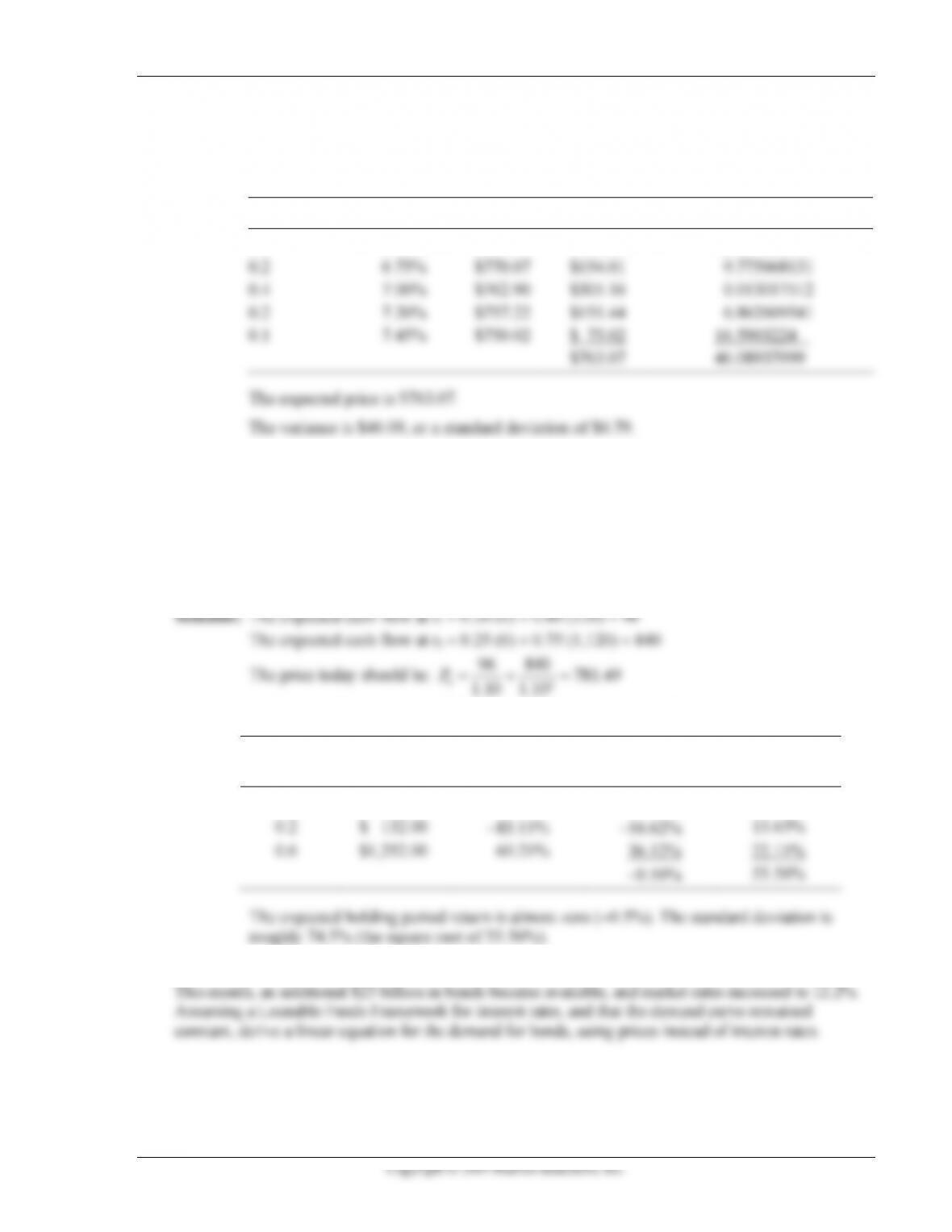
1. You own a $1,000-par zero-coupon bond that has 5 years of remaining maturity. You plan on selling
the bond in one year and believe that the required yield next year will have the following probability
distribution:
Probability
Required Yield
0.1
6.60%
0.2
6.75%
0.4
7.00%
0.2
7.20%
0.1
7.45%
Chapter 4: Why Do Interest Rates Change? 19
a. What is your expected price when you sell the bond?
b. What is the standard deviation?
Solution:
Probability
Required Yield
Price
Prob Price
Prob (Price − Exp. Price)2
0.1
6.60%
$774.41
$ 77.44
12.84776241
0.2
6.75%
$770.07
$154.01
9.775668131
0.4
7.00%
$762.90
$305.16
0.013017512
0.2
7.20%
$757.22
$151.44
6.862609541
0.1
7.45%
$750.02
$ 75.02
16.5903224
$763.07
46.08937999
The expected price is $763.07.
The variance is $46.09, or a standard deviation of $6.79.
2. Consider a $1,000-par junk bond paying a 12% annual coupon. The issuing company has 20% chance
of defaulting this year; in which case, the bond would not pay anything. If the company survives the
first year, paying the annual coupon payment, it then has a 25% chance of defaulting in the second
year. If the company defaults in the second year, neither the final coupon payment nor par value of
the bond will be paid. What price must investors pay for this bond to expect a 10% yield to maturity?
At that price, what is the expected holding period return? Standard deviation of returns? Assume that
periodic cash flows are reinvested at 10%.
02
1.10 1.10
At the end of two years, the following cash flows and probabilities exist:
Probability
Final Cash
Flow
Holding Period
Return
Prob HPR
Prob (HPR −
Exp. HPR)2
0.2
$ 0.00
−100.00%
−20.00%
19.80%
0.2
$ 132.00
−83.11%
−16.62%
13.65%
0.6
$1,252.00
60.21%
36.12%
22.11%
−0.50%
55.56%
The expected holding period return is almost zero (−0.5%). The standard deviation is
roughly 74.5% (the square root of 55.56%).
3. Last month, corporations supplied $250 billion in bonds to investors at an average market rate of 11.8%.
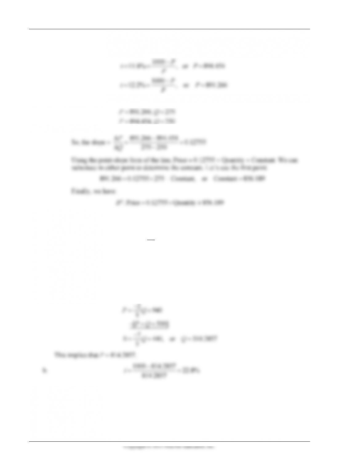
20 Mishkin/Eakins • Financial Markets and Institutions, Eighth Edition
Solution: First, translate the interest rates into prices.
1000
11.8% , or 894.454
P
iP
P
−
= = =
1000
12.2% , or 891.266
P
iP
P
−
= = =
We know two points on the demand curve:
891.266, 275
894.454, 250
PQ
PQ
==
==
So, the slope =
891.266 894.454 0.12755
275 250
P
Q
−
==
−
Using the point-slope form of the line, Price = 0.12755 Quantity + Constant. We can
substitute in either point to determine the constant. Let’s use the first point:
891.266 0.12755 275 + Constant, or Constant 856.189= =
Finally, we have:
: Price 0.12755 Quantity 856.189
d
B= +
4. An economist has estimated that, near the point of equilibrium, the demand curve and supply curve
for bonds can be estimated using the following equations:
2
: Price Quantity 940
5
: Price Quantity 500
d
s
B
B
−
=+
=+
a. What is the expected equilibrium price and quantity of bonds in this market?
b. Given your answer to part (a), which is the expected interest rate in this market?
Solution:
a. Solve the equations simultaneously:
2940
5
[ 500]
7
0 440, or 314.2857
5
PQ
PQ
QQ
−
=+
− = +
−
= + =
This implies that P = 814.2857.
b.
1000 814.2857 22.8%
814.2857
i−
==
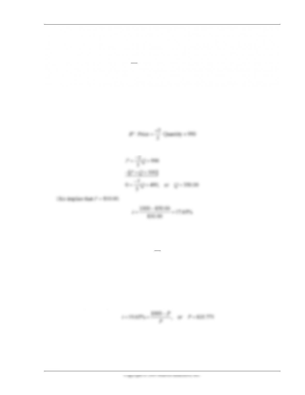
Chapter 4: Why Do Interest Rates Change? 21
5. As in Question 6, the demand curve and supply curve for bonds are estimated using the following
equations:
2
: Price Quantity 940
5
: Price Quantity + 500
d
s
B
B
−
=+
=
Following a dramatic increase in the value of the stock market, many retirees started moving money
out of the stock market and into bonds. This resulted in a parallel shift in the demand for bonds, such
that the price of bonds at all quantities increased $50. Assuming no change in the supply equation for
bonds, what is the new equilibrium price and quantity? What is the new market interest rate?
Solution:
The new demand equation is as follows:
2
: Price Quantity 990
5
d
B−
=+
Now, solve the equations simultaneously:
2990
5
[ 500]
7
0 490, or 350.00
5
PQ
PQ
QQ
−
=+
− = +
−
= + =
This implies that P = 850.00.
1000 850.00 17.65%
850.00
i−
==
6. Following Question 5, the demand curve and supply curve for bonds are estimated using the
following equations:
Bd: Price =
2 Quantity 990
5
−+
Bs: Price = Quantity + 500
As the stock market continued to rise, the Federal Reserve felt the need to increase the interest rates.
As a result, the new market interest rate increased to 19.65%, but the equilibrium quantity remained
unchanged. What are the new demand and supply equations? Assume parallel shifts in the equations.
Solution: Prior to the change in inflation, the equilibrium was Q = 350.00 and P = 850.00. The new
equilibrium price can be found as follows:
1000
19.65% , or 835.771
P
iP
P
−
= = =
22 Mishkin/Eakins • Financial Markets and Institutions, Eighth Edition
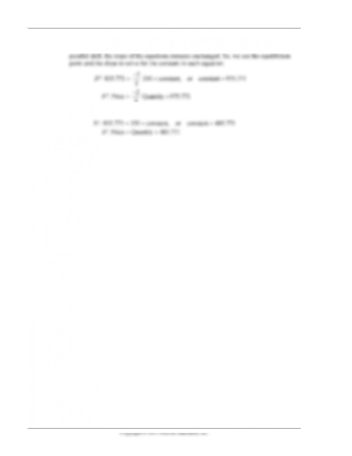
This point (350, 835.771) will be common to both equations. Further since the shift was a