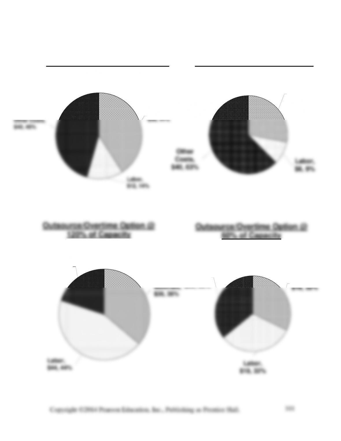
Labor,
$12, 14%
Other Costs,
$40, 45%
Materials,
$36, 41%
Other
Costs,
$40, 63%
Labor,
$6, 9%
Materials,
$18, 28%
Labor,
$44, 44%
Other Costs,
$20, 20%
Materials,
$36, 36%
Labor,
$18, 32%
Materials,
$18, 32%
Other
Costs,
$20, 36%
COST BEHAVIOR OF CAPACITY COSTS (Millions)
Build Option @ 120% of Capacity
Build Option @ 60% of Capacity
Outsource/Overtime Option @
120% of Capacity
Outsource/Overtime Option @
60% of Capacity
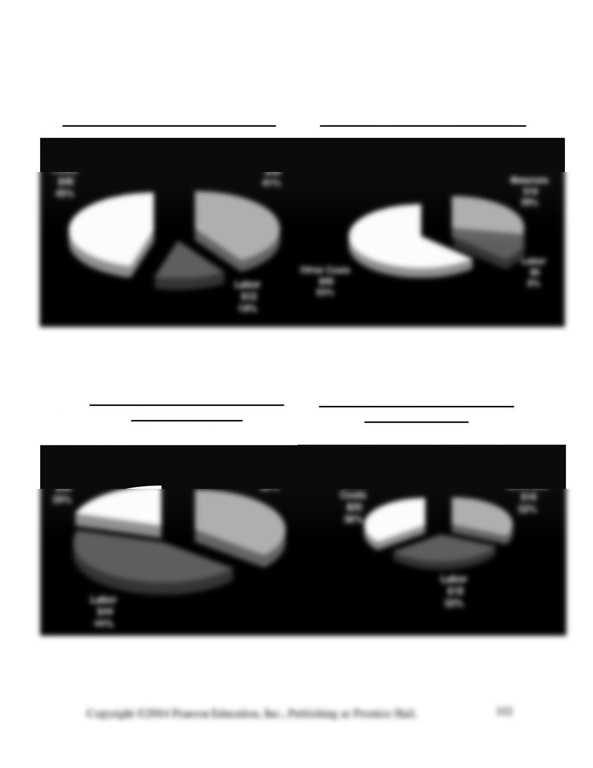
COST BEHAVIOR OF CAPACITY COSTS (Millions)
Build Option @ 120% of Capacity
Build Option @ 60% of Capacity
Outsource/Overtime Option @
120% of Capacity
Outsource/Overtime Option @
60% of Capacity
Build @ 120%
Labor
$12
14%
Materials
$36
Other
Costs
Build @ 60%
Labor
$6
9%
Other Costs
$40
63%
Outsource @120%
Labor
$44
44%
Materials
$36
36%
Other
Costs
$20
20%
Outsource @ 60%
Materials
$18
32%
Labor
$18
32%
Other
Costs
$20
36%
3-40 (30-35 min.)
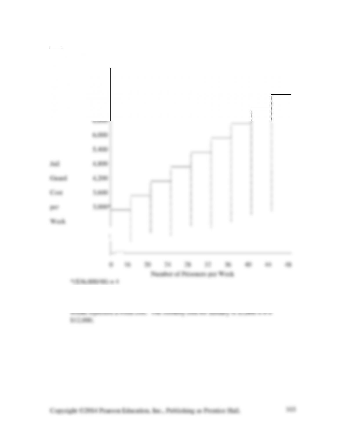
1. The graph of weekly planned cost of jail guards versus number of prisoners
shows that this cost is a step cost beyond 16 prisoners.
$7,800
7,200
2. In January up to 16 prisoners are expected; therefore, $3,000 per week should be
planned for jail guard costs. This represents the minimum staffing level, and
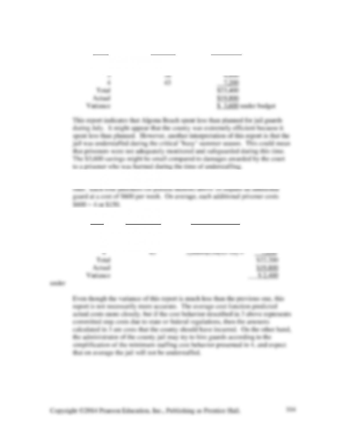
3. Actual Minimum
Week Prisoners Guard Cost
1 25 $ 4,800
2 38 6,600
4. The $3,000 fixed amount is the total weekly salary paid to the permanent guard
5. Week Actual Prisoners Minimum Guard Cost
1 25 $ 3,000+$150(25-16) = $ 4,350
2 38 3,000+$150(38-16) = 6,300
3 26 3,000+$150(26-16) = 4,500
3-41 (25-30 min.)
2. If the cost measurements are reliable, then the audit office is overstaffed by
approximately five auditors. Each auditor should be able to process 4 weeks × 5
auditors.
3. The variance may be due to inefficiency of the auditors, improperly trained or
inexperienced auditors, inaccuracy of the cost measures, a batch of unusually
4. Besides number of returns, alternative cost drivers might include number of
3-42 (10-15 min.) One possible cost driver is shown, with cost behavior with respect
to the cost driver in parentheses. Other cost drivers are also possible.
a. Airplane fuel — Flight miles (variable)
3-43 (25-30 min.)
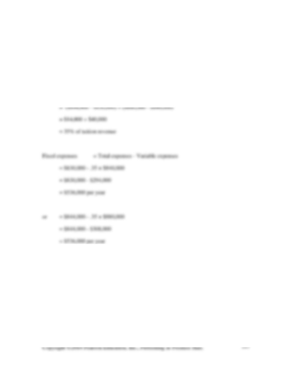
The first temptation may be to measure the cost behavior with the high-low
method, using the cost and activity levels from 20X7 and 20X9 since they are the lowest
and highest cost and activity levels given. However, Dr. Hyde has indicated that drug test
procedures are both more numerous and more complex than they were in the past.
raw monthly data are probably available. One recommendation would be to disregard
data from the first two years and to use monthly data from the third year to measure
current cost behavior. It could well be that this analysis will indicate a need for the price
increase demanded by Dr. Hyde.
Cost of Test Procedures
0
20,000
40,000
60,000
80,000
100,000
120,000
140,000
160,000
0100 200 300 400 500 600 700
Num ber of Procedures
Cost in Dollars
Cost
3-44 (30-35 min.)
The data should be used to first determine variable expenses as a function
(percentage) of tuition revenue. Then fixed expenses can be calculated. Since only two
data points are available, the high-low method is the appropriate approach.
Variable expenses = Change in expenses ÷ Change in revenues
Income for 2013 may be predicted as follows:
OCEANVIEW SCHOOL
Projected Income
For the Year Ending August 31, 2013
Tuition revenue $830,000
Less: Variable expenses (.35 × $830,000) $290,500
Fixed expenses 536,000
826,500
Net Income $ 3,500
Or, Net Income = Tuition revenue – variable expenses – fixed expenses
= $830,000 – .35× $830,000 – $536,000
= .65 × $830,000 – $536,000 = $3,500
Break-even tuition revenue may be found by setting Net Income = 0 and solving for the
unknown tuition revenue, TR, as below:
0 = TR -.35TR – $536,000
0 = .65TR – $527,600
$536,000 = .65TR
TR = $824,615 at break-even (rounded)
3-45 (20-25 min.)
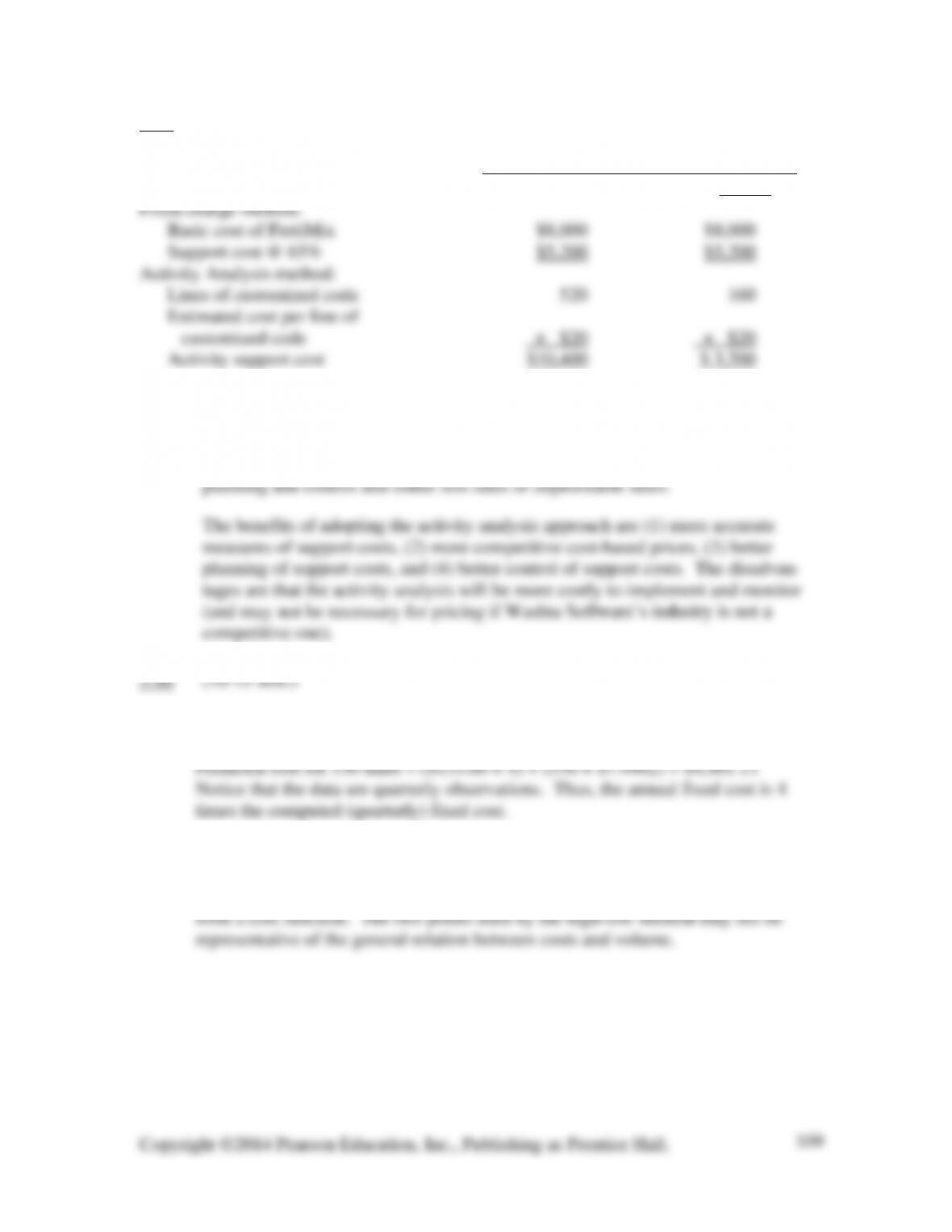
1. Support cost measurement:
Customer
Mystical Plants Todal Blooms
2. The activity analysis approach indicates that products requiring large amounts of
customizing incur much more support cost than those that require relatively little
customizing. The old approach leads to distorted costs that might lead to poor
1. Variable cost/unit = ($1,124 – $640) (133 – 68) = $484 65 = $7.4462
Fixed cost = $1,124 – (133 × 7.4462) = $1,124 – $990.34 = $133.66
2. Predicted cost for 530 units = ($347 × 4) + (530 × $5.76) = $4,440.80
3. The regression analysis gives better cost estimates because it uses all the data to
3-47 (35-40 min.)
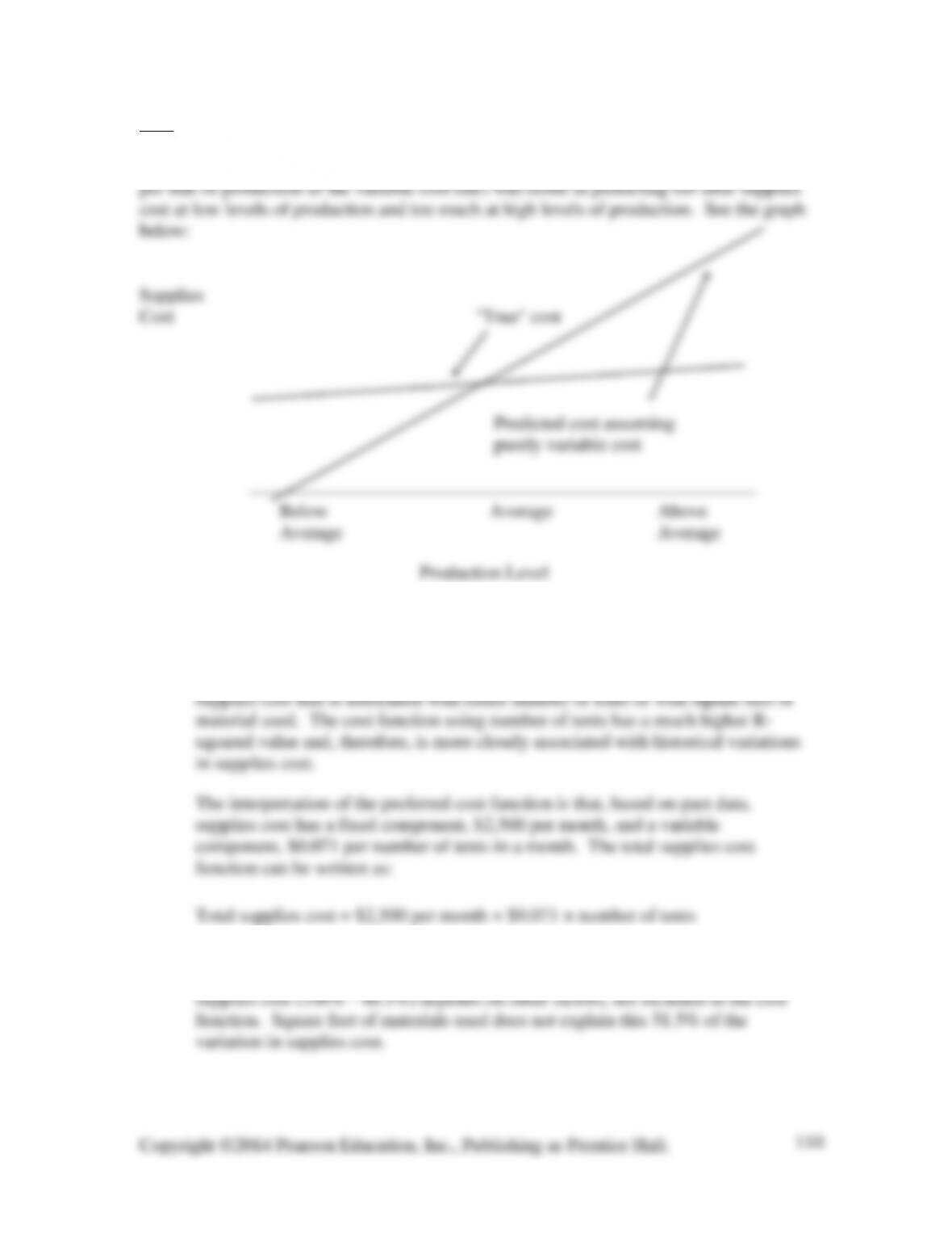
If supplies cost is at least partly fixed with regard to production volume, then
treating supplies cost as if it were purely variable (e.g., using the average supplies cost
1. The preferred cost function uses “number of tents” as the cost driver for supplies
cost. Although many other statistical criteria could be (should be) used to make
this determination, this choice is based on the relative R-squared values. The R-
squared measures the amount (percentage) of fluctuation (variation) in historical
2. Approximately 48.5% of the variation in historical supplies cost is associated with
variations in square feet of materials. The remaining 51.5% of variation in
3-48 (40-45 min. unless data supplied by instructor, then 25-30 min.)
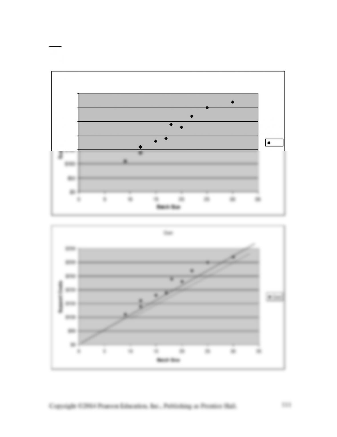
1. The accompanying graphs can be used to discuss requirements 2-4.
Cost
$0
$50
$100
$150
$200
$250
$300
$350
0 5 10 15 20 25 30 35
Batch Size
Support Costs
Cost
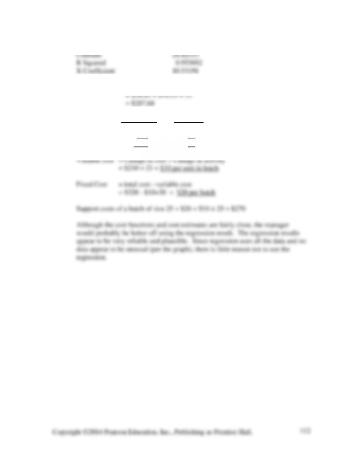
2. Regression Output:
3. Support costs = fixed cost + variable cost
4. Support cost Batch size
High Level $320 30
Low Level 110 9
Difference $210 21