
CHAPTER 3
COVERAGE OF LEARNING OBJECTIVES
LEARNING
OBJECTIVE
FUNDA-
MENTAL
ASSIGN-
MENT
MATERIAL
CRITICAL
THINKING
EXERCISES
AND
EXERCISES
PROBLEMS
CASES,
NIKE 10K,
EXCEL,
COLLAB., &
INTERNET
EXERCISES
LO1: Explain
management
influences on cost
behavior.
26, 33
39
52, 56
LO2: Measure
and
mathematically
express cost
functions and use
them to predict
costs.
27, 29, 30, 31,
34
35, 36, 37
38
39, 40, 44, 41,
46
48, 50, 51
57, 56, 58
LO3: Describe
the importance of
activity analysis
for measuring
cost functions.
A1,B1
42,45
53, 55
LO4: Measure
cost behavior
using the
engineering
analysis, account
analysis, high-
low, visual-fit,
and least-squares
regression
methods.
A2,B2
28, 29, 30, 34,
35
36, 37, 38
43, 46, 47
48, 49, 51
54, 58
CHAPTER 3
Measurement of Cost Behavior
3-A1 (25-30 min.)
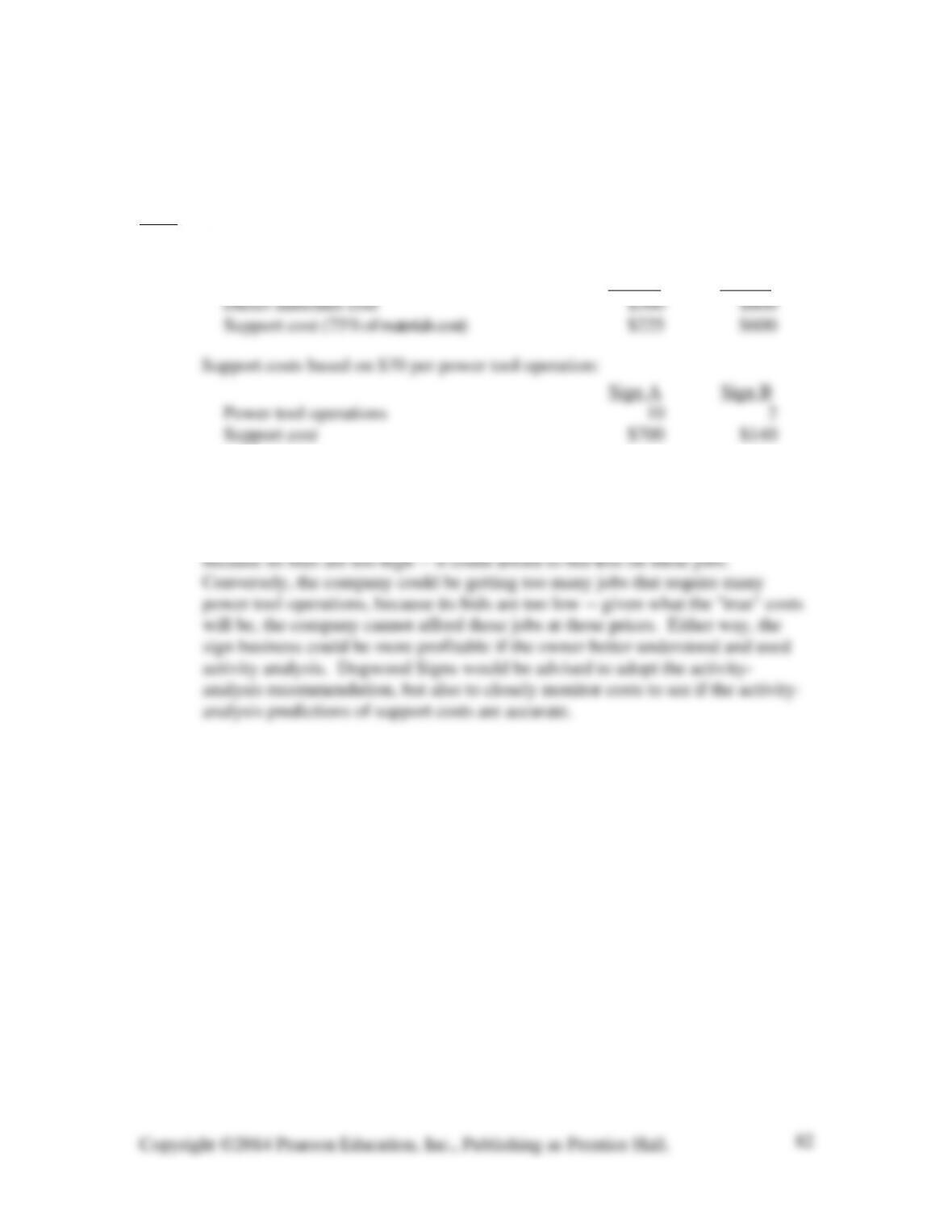
1. Support costs based on 75% of the cost of materials:
Sign A Sign B
2. If the activity analysis is reliable, by using the current method, Dogwood Signs is
predicting too much cost for signs that use few power tool operations and is
predicting too little cost for signs that use many power tool operations. As a
result the company could be losing jobs that require few power tool operations
3-A2 (25-30 min.)
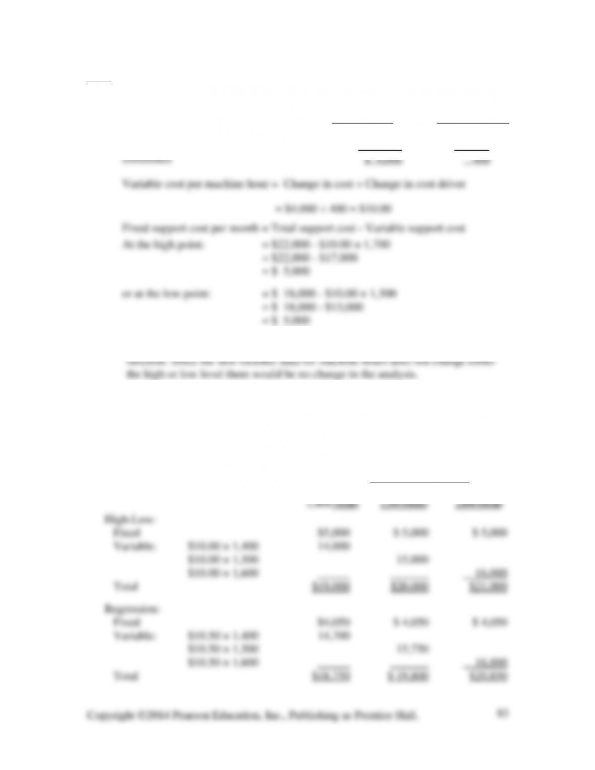
1. High-Low Method:
Support Cost Machine Hours
High month = May $22,000 1,700
Low month = September 18,000 1,300
2. The high-low method uses the high and low activity levels to determine the cost
3. The regression analysis results differ from the results of the high-low method.
As a result, estimates of total support cost may differ considerably depending on
the expected machine hour usage. For example, consider the following support
cost estimates at three levels of machine hour usage (all within the relevant
range):
Machine Hour Usage
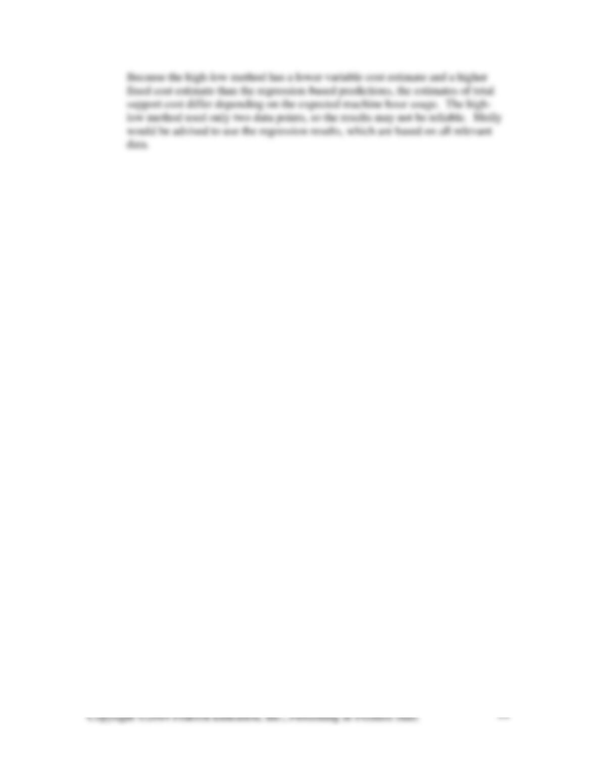
Because the high-low method has a lower variable cost estimate and a higher
fixed cost estimate than the regression-based predictions, the estimates of total
support cost differ depending on the expected machine hour usage. The high-
low method used only two data points, so the results may not be reliable. Molly
would be advised to use the regression results, which are based on all relevant
data.
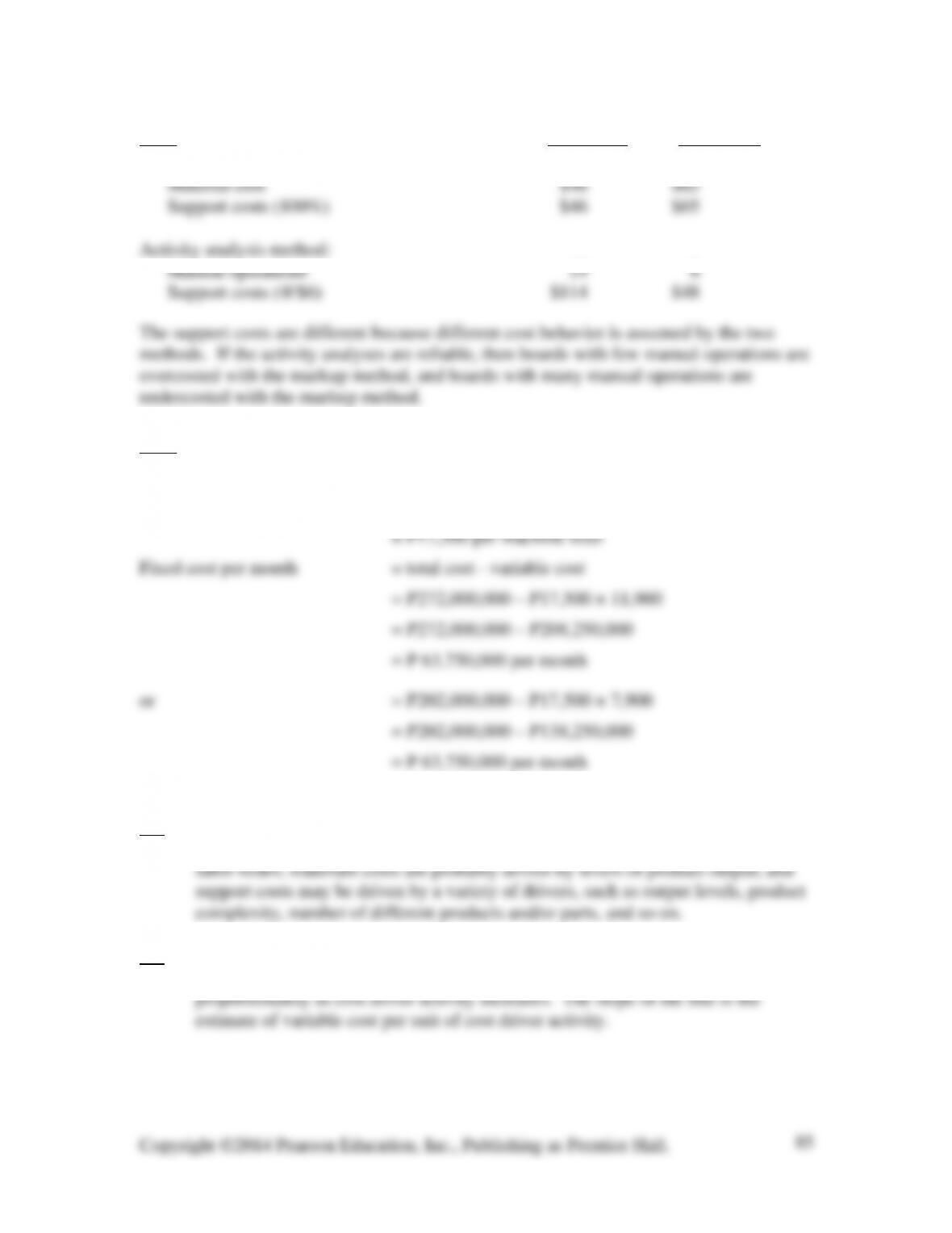
3-B1 (25-30 min.) Board Z15 Board Q52
Mark-up method:
3-B2 (25-30 min.)
Variable cost per machine hour = Change in Repair Cost ÷ Change in Machine Hours
= (P272,000,000 – P202,000,000) ÷ (11,900 – 7,900)
3-1 A cost driver is any output measure that is believed to cause costs to fluctuate in a
predictable manner. For example, direct labor costs are probably driven by direct
3-2 Linear cost behavior assumes that costs behave as a straight line. This line is
anchored by an intercept, or fixed cost estimate, and total costs increase
3-3 Whether to categorize a step cost either as a fixed cost or as a variable cost
depends on the “size” of the steps (height and width) and on the desired accuracy
of the description of step cost behavior. If the steps are wide, covering a wide
3-4 Mixed costs are costs that contain both fixed and variable elements. A mixed cost
has a fixed portion that is usually a cost per time period. This is the minimum
3-5 In order to achieve the goals set for the organization, management makes critical
choices — choices that guide the future activities of the organization. These
3-6 Some fixed costs are called capacity costs because the levels of these fixed costs
3-7 Committed fixed costs are costs that are often driven by the planned scale of
operations. These costs typically cannot be changed easily or quickly without
drastically changing the operations of the organization. Typical committed fixed
costs include lease or mortgage payments, property taxes, and long-term
3-8 Committed fixed costs are the most difficult to change because long-term
commitments generally have been made. These long-term commitments may
3-9 An organization’s capacity generally determines its committed fixed costs.
Management’s choice is the main influence on discretionary fixed costs. Both
3-10 Both planning for and controlling discretionary costs are important. It is hard to
say that one is more important than the other, but certainly effective use of
3-12 Incentives to control costs are means of making cost control in the best interests
of the people responsible for making cost expenditures. A simple example will
illustrate the use of incentives to control costs. Assume that you are an executive
3-13 Use of cost functions, or algebraic representations of cost behavior, allows cost
analysts or management to build models of the organization’s cost behavior.
3-14 A “plausible” cost function is one that is intuitively sound. A cost function is
plausible if a knowledgeable analyst can make sound economic justifications why
a particular cost driver could cause the cost in question. A “reliable” cost function
3-15 Activity analysis identifies underlying causes of cost behavior (appropriate cost
3-16 Engineering analysis is a method of identifying and measuring cost and cost
driver relationships that does not require the use of historical data. Engineering
analysis proceeds by the use of interviews, experimentation, and observation of
3-17 There are four general methods covered in this text to measure mixed costs using
historical data: (1) account analysis, (2) high-low, (3) visual fit, and (4)
regression.
• Account analysis looks to the organization’s cost accounts and classifies each
3-18 Engineering analysis and account analysis often are combined. One of the
problems of account analysis is that historical data may contain past
3-19 The strengths of the high-low method are also its weaknesses — the method is
simple to apply since it does not require extensive data or statistical
sophistication. This simplicity also means that the method may not be reliable
3-20 The cost-driver level should be used to determine the two data points to be used to
3-21 Regression analysis is usually preferred to the high-low method (and the visual-fit
method) because regression analysis uses all the relevant data and because easy-
3-22 This is a deceptive statement, because it is true on the face of it, but regression
also has many pitfalls for the unwary. Yes, regression software provides useful
output that can be used to evaluate the reliability of the measured cost function. If
3-23 Plotting data helps to identify outliers, that is, observations that are unusual and
3-24 R2 is a goodness-of-fit statistic that describes the percentage of variation in cost
explained by changes in the cost driver.
3-25 Control of costs does require measurement of cost behavior, either what costs
have been or what costs should be. Problems of work rules and the like may
3-26 Both depreciation and research and development costs are fixed costs because
they are independent of the volume of operations. Depreciation is generally a
3-27 Decision makers should know a product’s cost function if their decisions affect
the amount of product produced. To know the cost impact of their decisions,
3-28 Regression analysis is a statistical method of fitting a cost-function line to
observed costs. It is objective; that is, each cost analyst would come up with the
1. The scales used for both axes are incorrect. The space between equal intervals in
number of orders and order-department costs should be the same.
2. The visual-fit line is too high, and the slope is too steep. It appears that the line
has been purposely drawn to pass through the (100,450) data point and the $200
3. The total cost for 90 orders is wrong. Either the fixed costs should be expressed in
thousands of dollars or the unit variable costs should be $2,000 per order. Even if
the derived total cost function was accurate, the resulting cost prediction is
incorrect. The formula should be expressed as:
Total cost (thousands of dollars) = $200 + $2.50 × Number of orders processed, or
Total cost = $200,000 + $2,500 × Number of orders processed
This would result in a predicted total cost for 90 orders of:
Total cost (thousands of dollars) = $200 + $2.50 × 90 = $425, or
Total cost = $200,000 + $2,500 × 90 = $425,000.
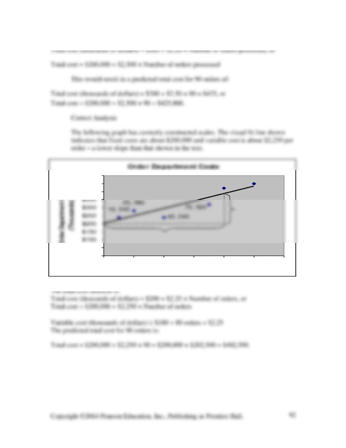
Correct Analysis
The following graph has correctly constructed scales. The visual fit line shown
indicates that fixed costs are about $200,000 and variable cost is about $2,250 per
order – a lower slope than that shown in the text.
Order Department Costs
10, 240
20, 280
100, 450
80, 420
40, 240
70, 320
$-
$50
$100
$150
$200
$250
$300
$350
$400
$450
$500
020 40 60 80 100 120
Orders Processed
Order Department Costs
(Thousands)
$180
3-30 (15-20 min.) Amounts are in millions.
1. 2010 2011
2. Change in operating expenses ÷ Change in revenues = Variable cost percentage
($93 – $85) ÷ ($154 – $74) = $8 ÷ $80 = .10 or 10%
3. Because fixed costs do not change, the entire additional total contribution margin
the $77.6 of fixed cost. But the additional $80 of sales revenue in 2011 generated
1. Fuel costs: $.40 × 16,000 miles per month = $6,400 per month.
3. Ambulance and EMT cost: $1,200 × (2,400/200) = $1,200 × 12 = $14,400
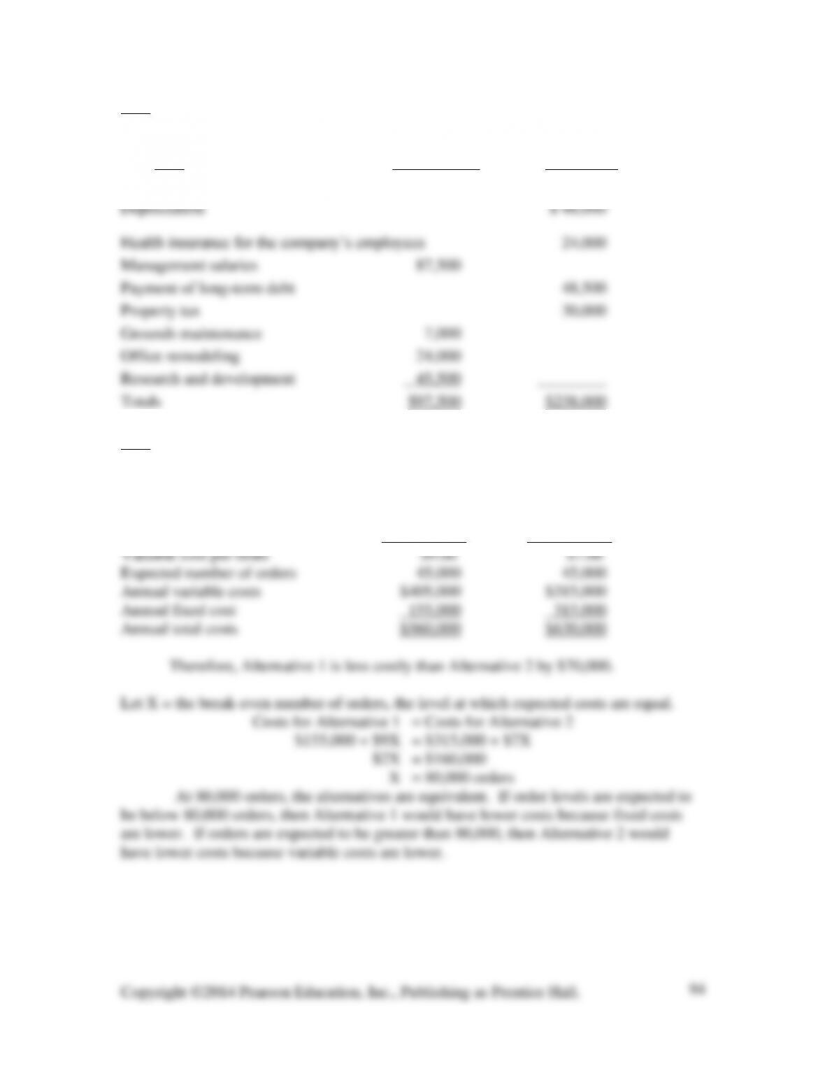
3-32 (10-15 min.) There may be some disagreement about these classifications, but
reasons for alternative classifications should be explored.
Cost Discretionary Committed
Advertising $21,000
3-33 (15-20 min.)
This problem extends the chapter analysis to preview short-run decision making
and capital budgeting. This problem ignores taxes, investment cost, and the time value of
money, which are covered in Chapter 11.
Alternative 1 Alternative 2
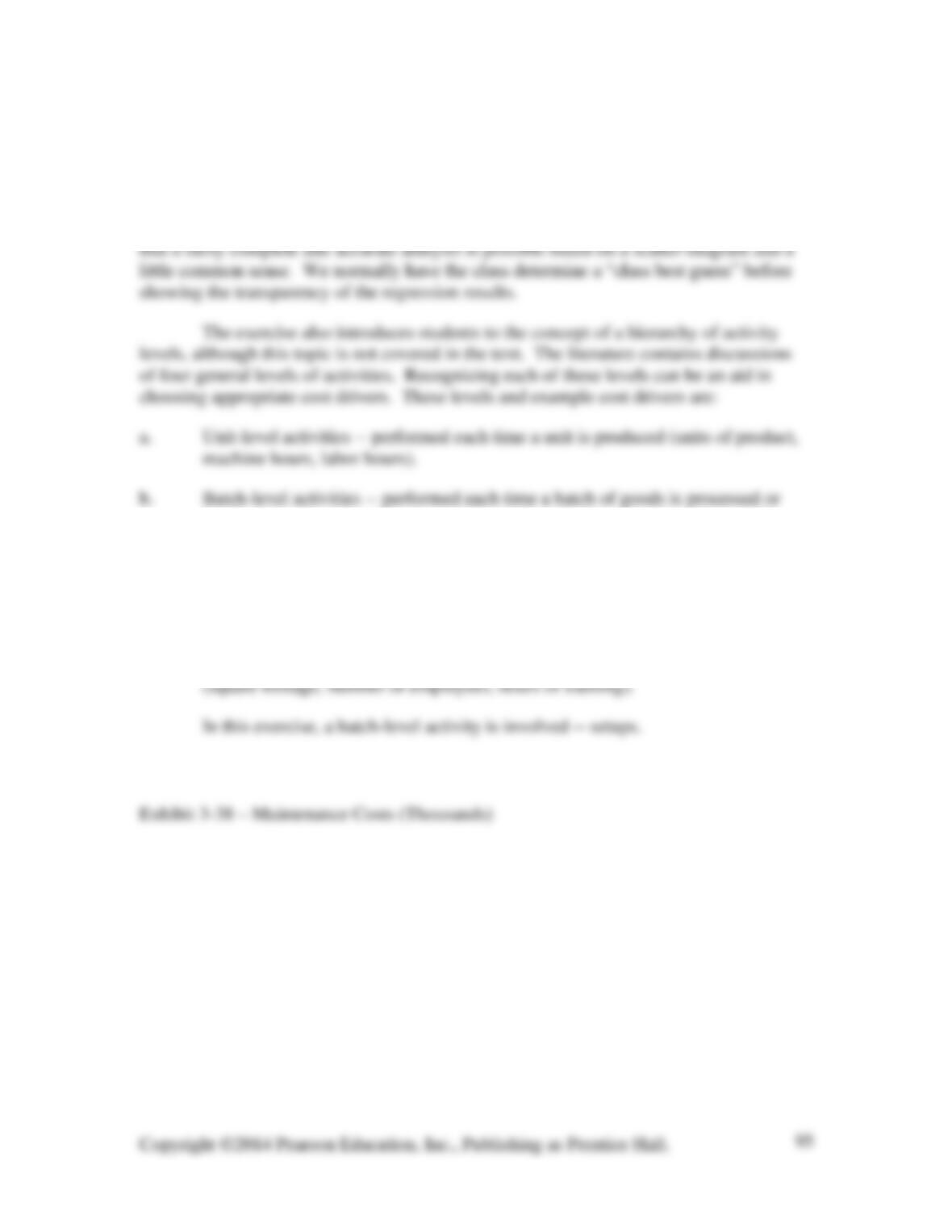
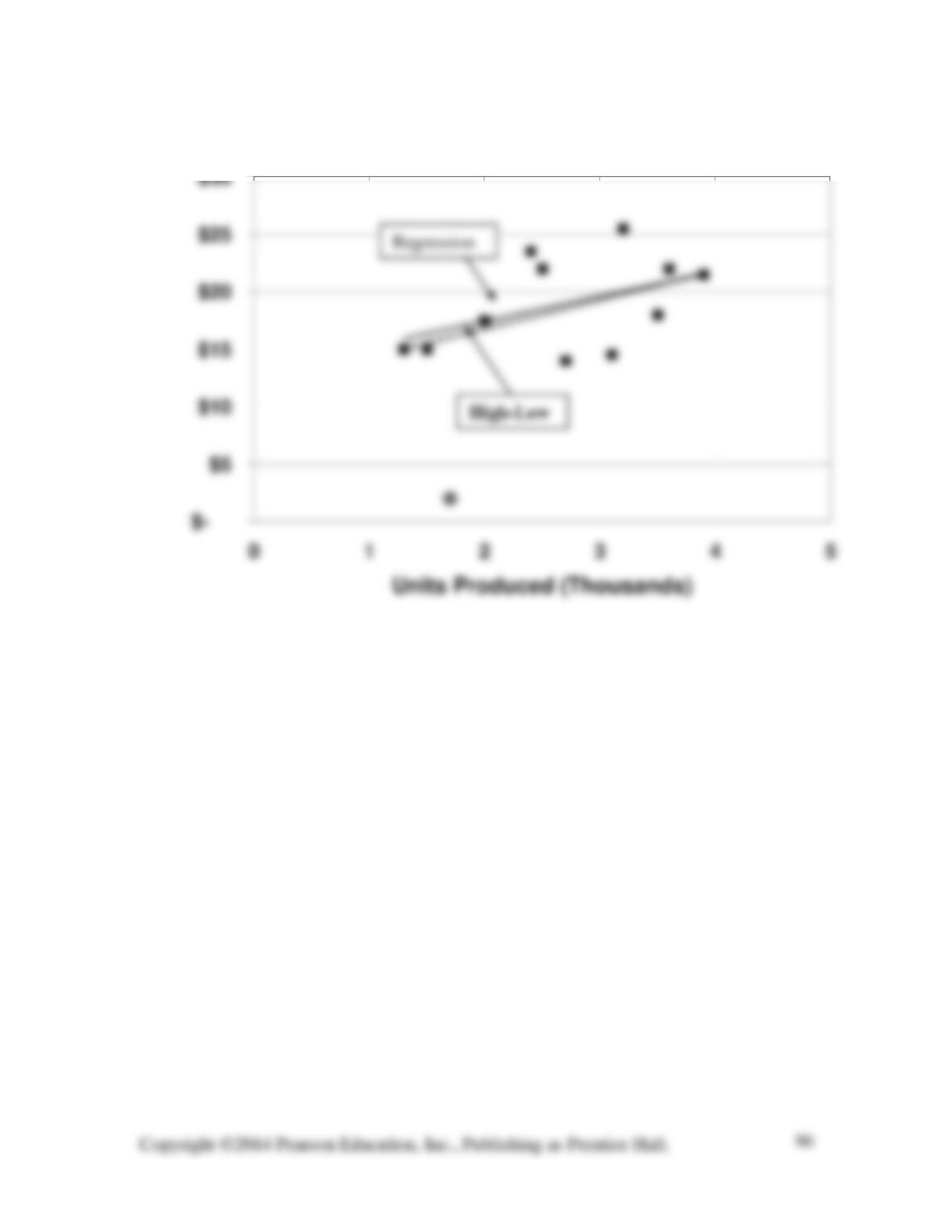
3-34 (20-25 min.) A master of the scatter-diagrams with least-square regression lines
and high-low lines appears in Exhibit 3-38 on the following page.
This exercise enables a comparison of the high-low and visual-fit methods of
decomposing mixed-costs into fixed and variable parts. Students find it interesting to
compare their best guesses to the least-squares regression results. They find it interesting
handled (number of orders processed, number of setups, number of material
moves).
c. Product-level activities — performed as needed to support the production of each
different type of product (number of tests, number of parts, number of
engineering change notices, hours of design time, number of inspections).
d. Facility-level activities — sustain a facility’s general manufacturing process
$-
$5
$10
$15
$20
$25
$30
0 1 2 3 4 5
Units Produced (Thousands)
High-Low
Regression
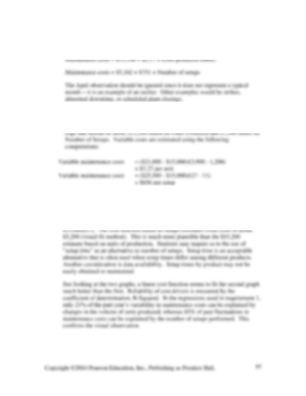
1. Student answers will vary somewhat. Least-squares regression lines are given as a
standard for comparison. Based on regression, the cost functions are:
2. The high-low method uses only the highest and lowest activity levels. Note that,
if one is using a scatter diagram, the high-low method can be used without
knowing the exact figures. Fixed cost can be easily estimated using a straight
3. Both cost drivers appear, on the surface, to be plausible. However, if
maintenance activity is primarily associated with a “batch–level” activity such as
setups, the setup driver is preferred. Of the three costs associated with
maintenance activity, supplies and energy are probably variable, so salaries are
the primary fixed costs. The monthly salary of two mechanics is $4,167 [(2 ×
3-35 (15-20 min.) The total cost for the month is $1,730 + (5 × $1,250) = $7,980,
based on the following cost function information:
Cost Fixed per month Variable per computer
Phone $ 60
3-36 (5 min.)
3-37 (5-10 min.)
Variable cost per ton = (£1,150,000 – £950,000) (55,000 – 35,000)
3-38 (10-15 min.)
The regression analysis results show that more was spent on building maintenance
in months of low production volume than in months of high volume. The
assistant controller erred in not thinking about the economic logic of this result.
3-39 (50-60 min.) (Masters of the line graph and pie charts appear on the next three
pages. Two versions of the pie charts are shown.)
1. The line graph shows the plot of the total cost for each of the two options at
various levels of capacity utilization. The outsource/ overtime option has a
2. Controlling risk usually means reducing the financial exposure of a company
when business conditions turn unfavorable. Companies attempt to control this
risk through various means — diversifying their product lines and markets and
reducing fixed (committed) costs or converting fixed costs into variable costs. In
3. Students’ answers to this question will vary depending on their attitudes toward
risk. This part of the problem helps students realize the value of different forms
of analysis. We use pie charts to demonstrate one form of analysis — tables can
also be used. The pie charts bring out the importance of fixed costs more readily
than the line graph. The four pie charts can be used to point out the value of
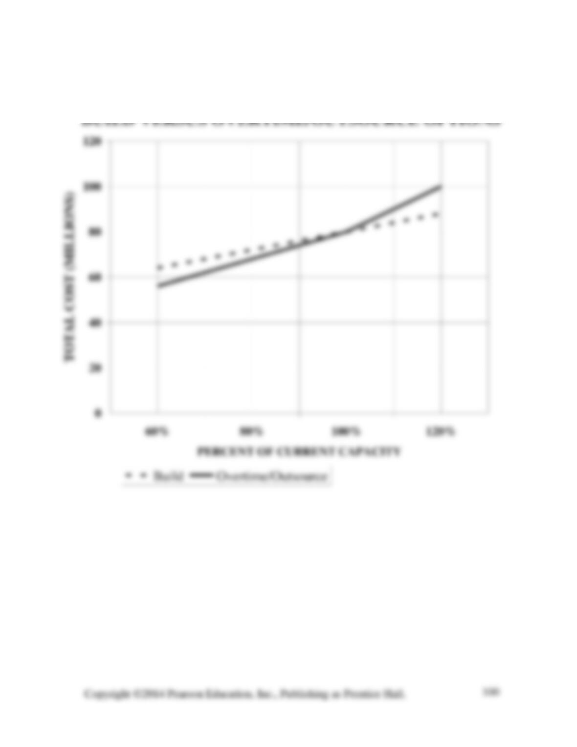
BUILD VERSUS OVERTIME/OUTSOURCE OPTIONS
0
20
40
60
80
100
120
60% 80% 100% 120%
PERCENT OF CURRENT CAPACITY
TOTAL COST (MILLIONS)
Build Overtime/Outsource