2-42 (15 min.)
a b
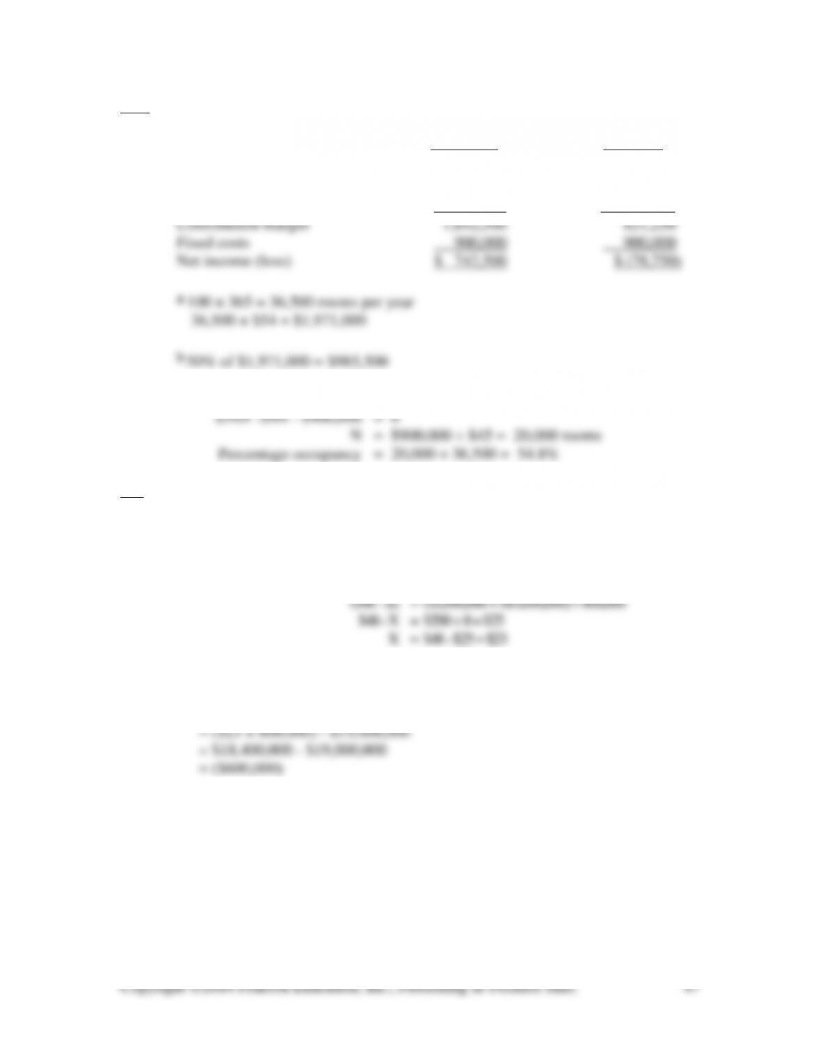
1. 100% Full 50% Full
Room revenue @ $54 $1,971,000 a $ 985,500 b
Variable costs @ $9 328,500 164,250
2. Let N = number of rooms rented
2–43 (15 min.)
1. $23. To compute this, let X be the variable cost that generates $1 million in
profits:
($48 – X ) × 800,000 – $19,000,000 = $1,000,000
2. Loss of $600,000:
($48 – $25) × 800,000 – $19,000,000
2-44 (15-20 min.)
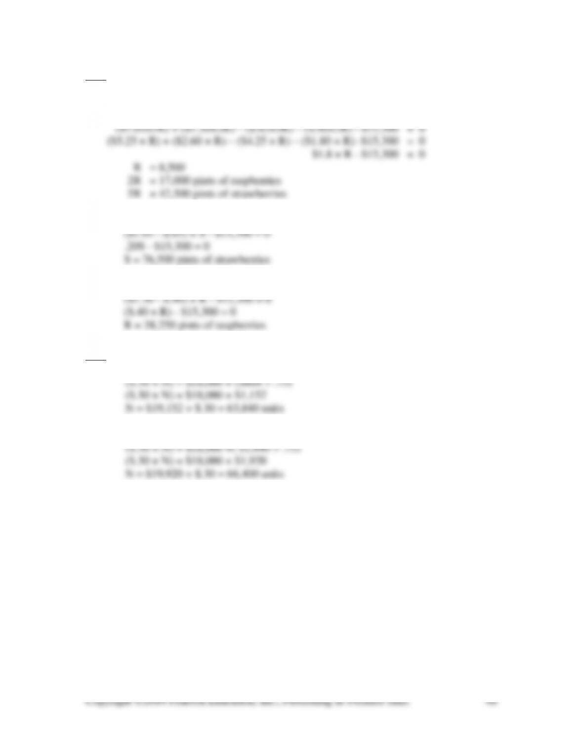
1. Let 2R = pints of raspberries and 5R = pints of strawberries
sales – variable expenses – fixed expenses = zero net income
2. Let S = pints of strawberries
3. Let R = pints of raspberries
2-45 (10 min.)
1. ($1.50 × N) – ($1.20 × N) – $18,000 = $864 ÷ (1 – .25)
2. ($1.50 × N) – ($1.20 × N) – $18,000 = $1,440 ÷ (1 – .25)
2-46 (15 min.)
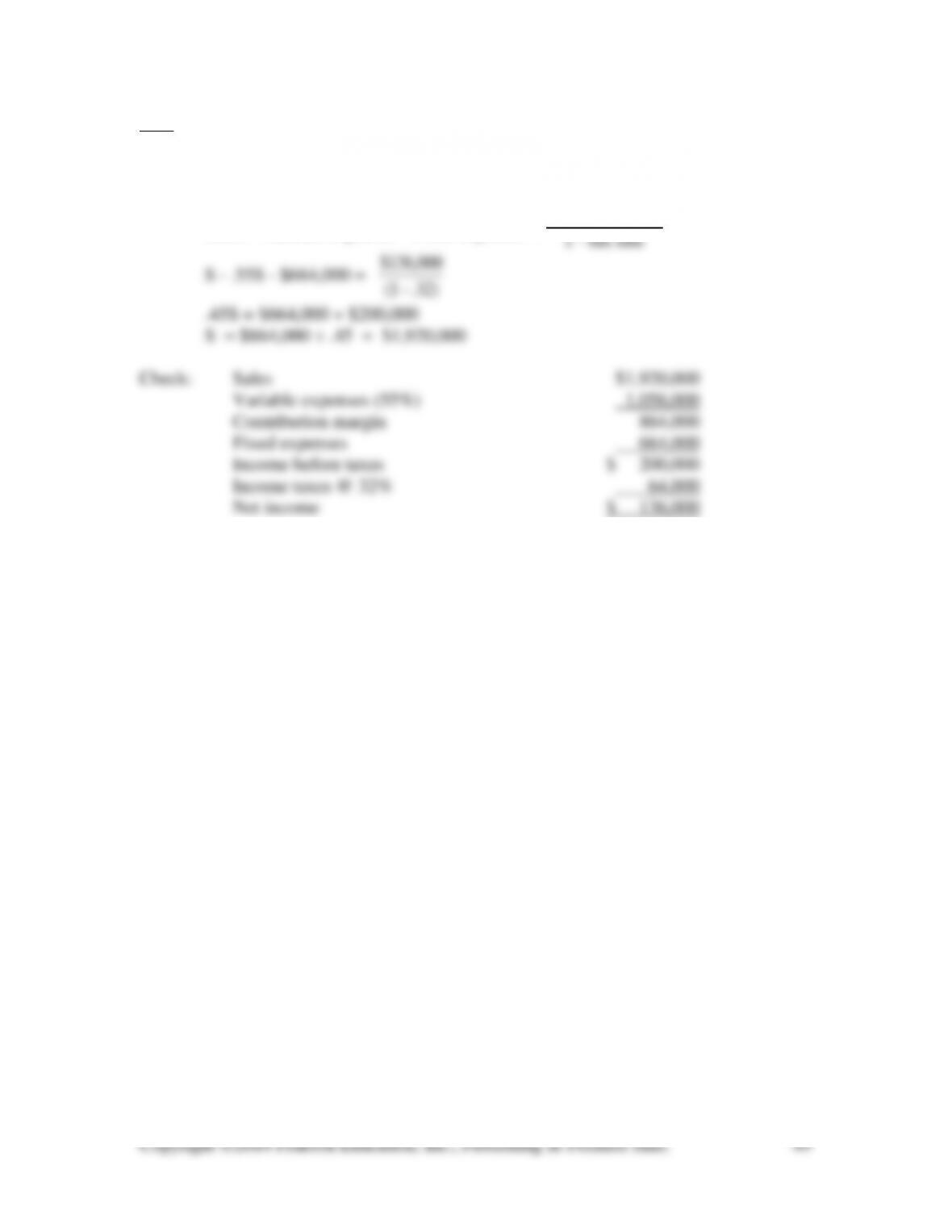
Several variations of the following general approach are possible:
Sales – Variable expenses – Fixed expenses =
Target after-tax
net income
2-47 (40-50 min.)
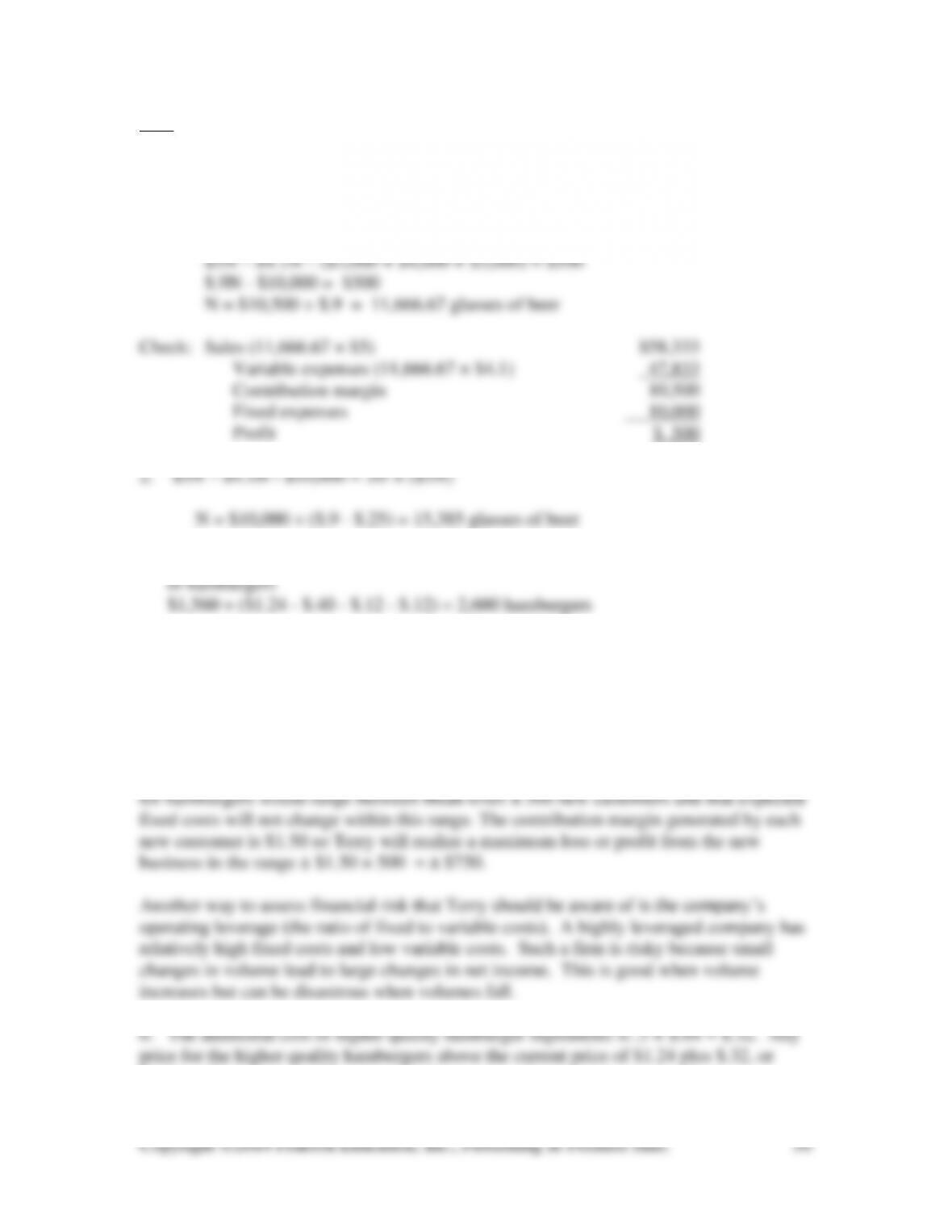
1. Several variations of the following general approach are possible:
Let N = Unit Sales.
Sales – Variable expenses – Fixed expenses = Profit
3. Fixed Cost ÷ (Sales price – cost of meat – cost of buns – cost of other ingredients) = #
4. (3,000 × $.60) + (4,800 × $.90) – $1,560 = $1,800 + $4,320 – $1,560 = $4,560 added profit
5. $1,560 ÷ ($.60 + $.90) = 1,040 new customers are needed to breakeven on the new
business.
A sensitivity analysis would help provide Terry with an assessment of the financial risks
associated with the new hamburger business. Suppose that Terry is confident that demand
$1.56, will improve profits, assuming the same number of customers purchase
hamburgers.
2-48 (30-40 min.)
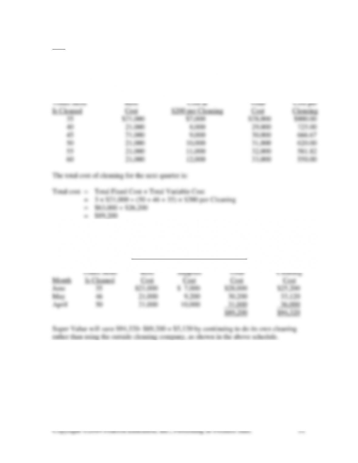
1. The cost of labor and equipment rent is fixed at $21,000 per month. Cleaning supplies
cost varies in proportion to the number of times the store is cleaned. The cost per
cleaning is $12,000 ÷ 60 = $200.
Number of Labor & Cleaning Supplies
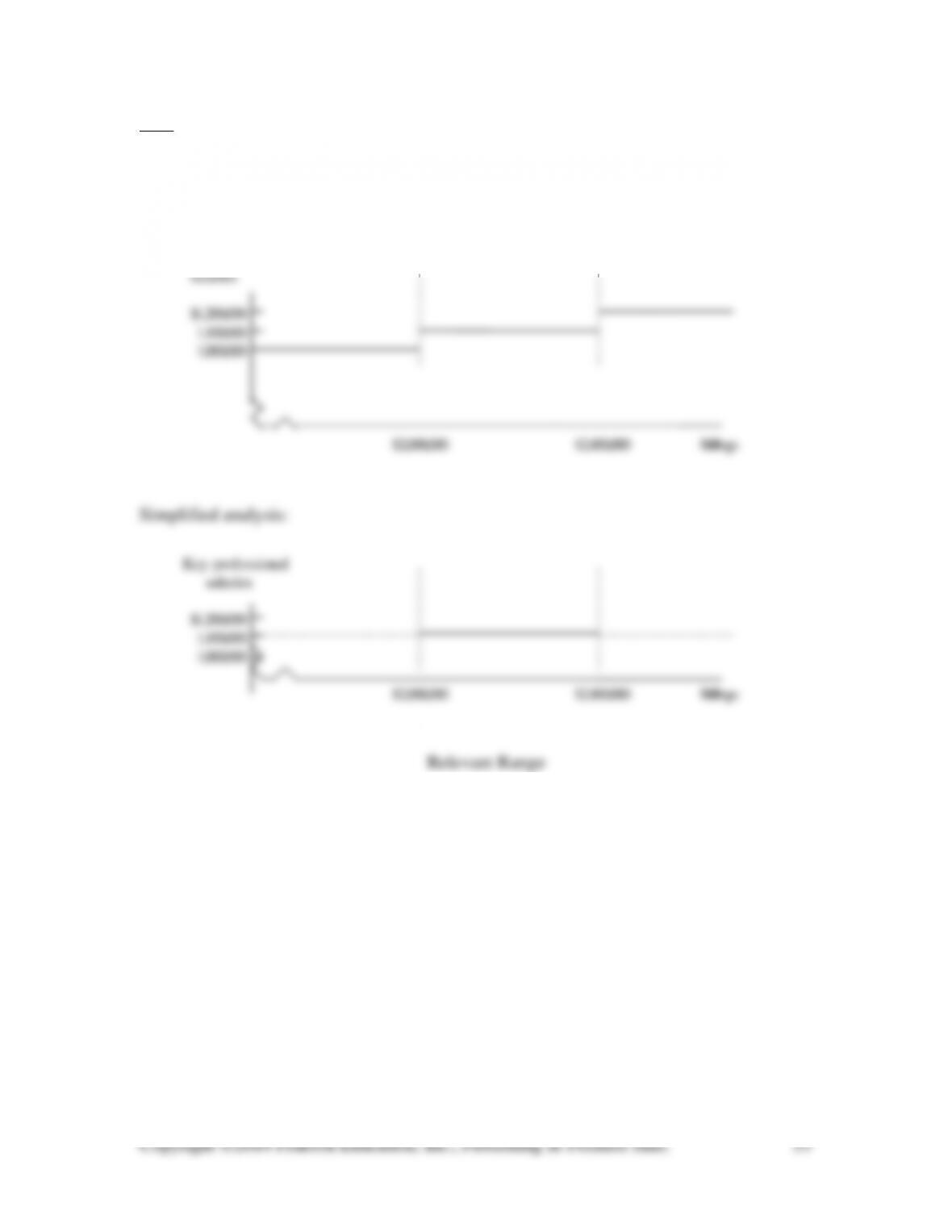
2. See the chart on the next page.
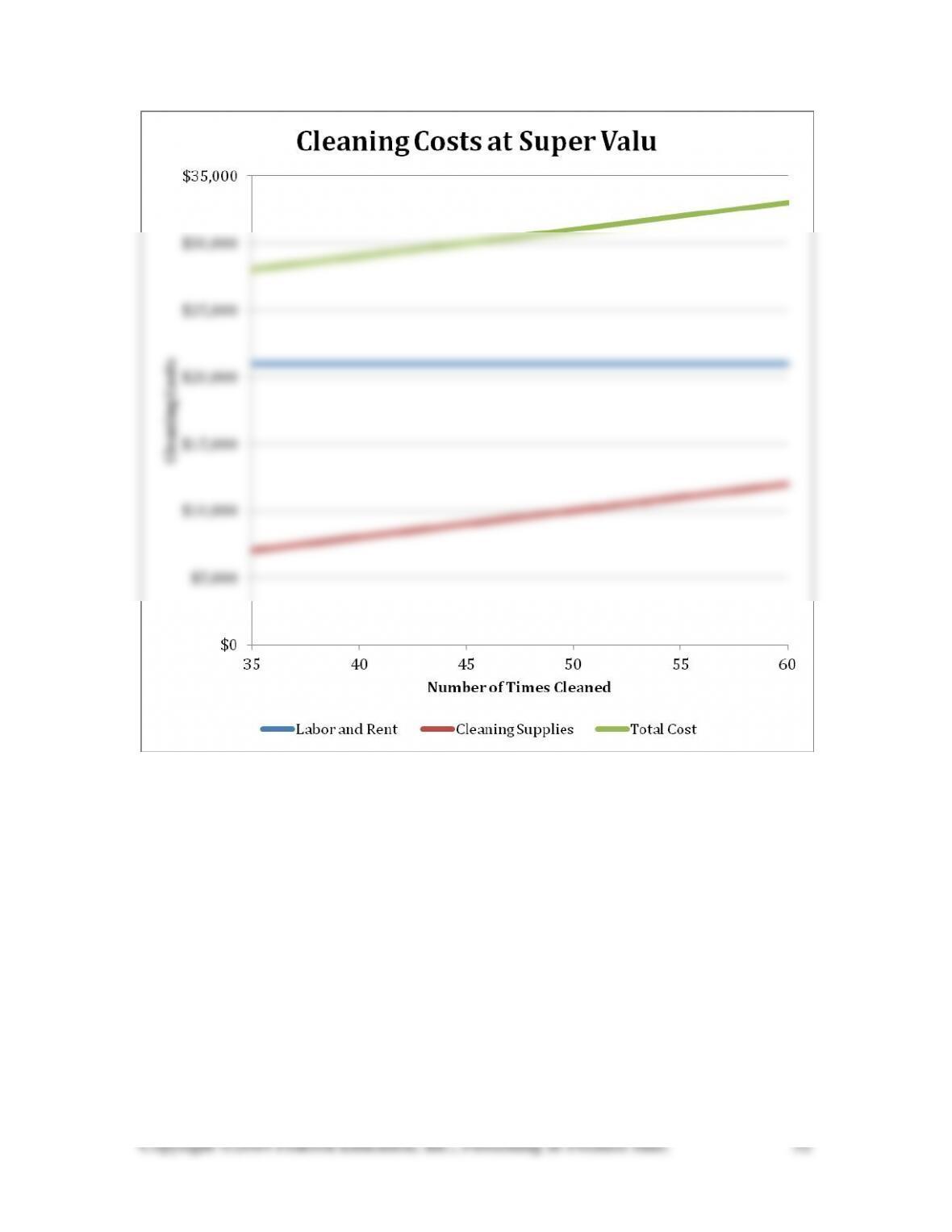
3.
Costs of Super Valu Cleaning Store
Number of Labor & Cleaning Outside
2-49 (10-15 min.)
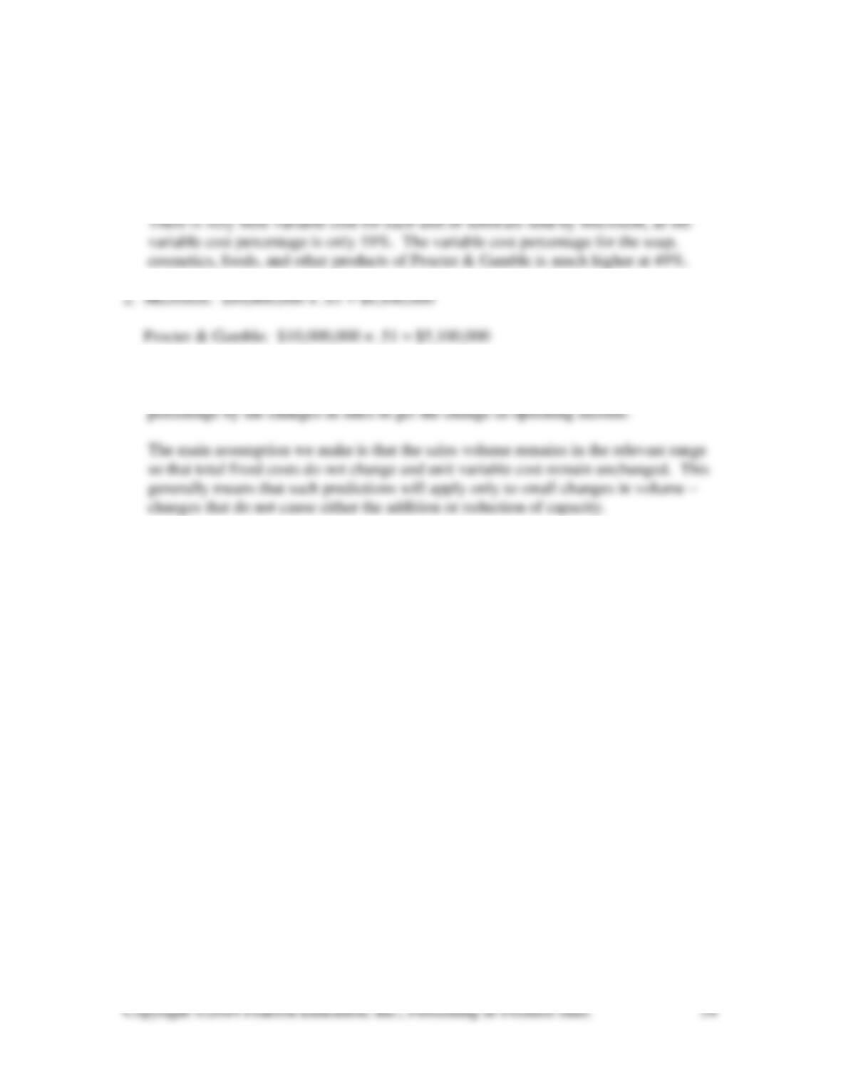
The budget for professional salaries for the coming year is $1,100,000.
Refined analysis:
Key professional
2-50 (15-20 min.)
1. Microsoft: ($60,420 – $11,598) ÷ $60,420 = .81 or 81%
Procter & Gamble: ($83,503 – $40,695) ÷ $83,503) = .51 or 51%
3. We know that the total contribution margin generated by any added sales will be
added to the operating income. Thus, we can simply multiply the contribution margin
2-51 (15-20 min.)
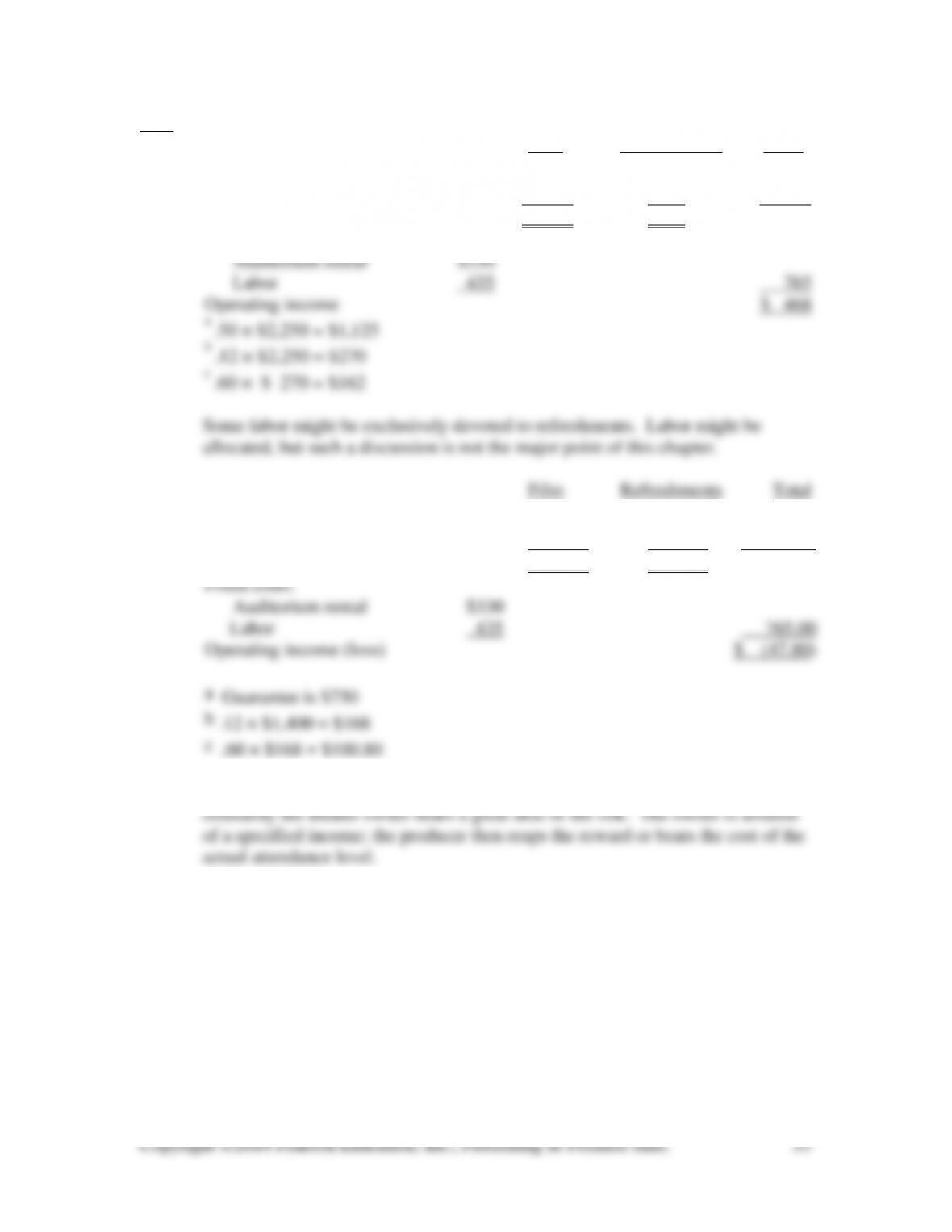
Film Refreshments Total
1. Revenue from admissions $2,250 $270 b $2,520
Variable costs 1,125 a 162 c 1,287
Contribution margin $1,125 $108 $1,233
Fixed costs:
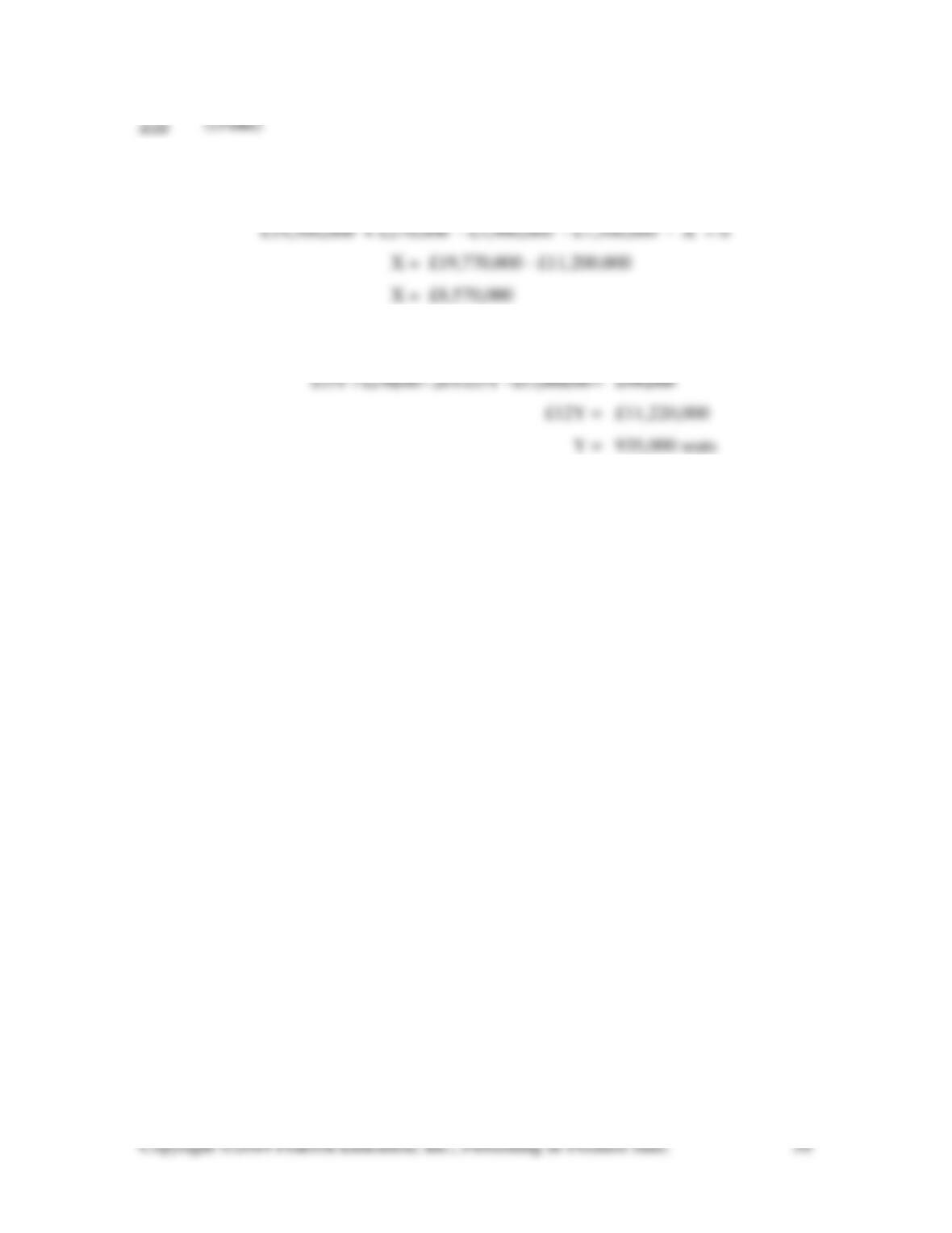
2. Revenue from admissions $1,400.00 $168.00b $1,568.00
Variable costs 750.00a 100.80c 850.80
Contribution margin $650.00 $ 67.20 $ 717.20
3. The offer would shift the risk completely to the movie producer, whereas
2–52 (15 min.)
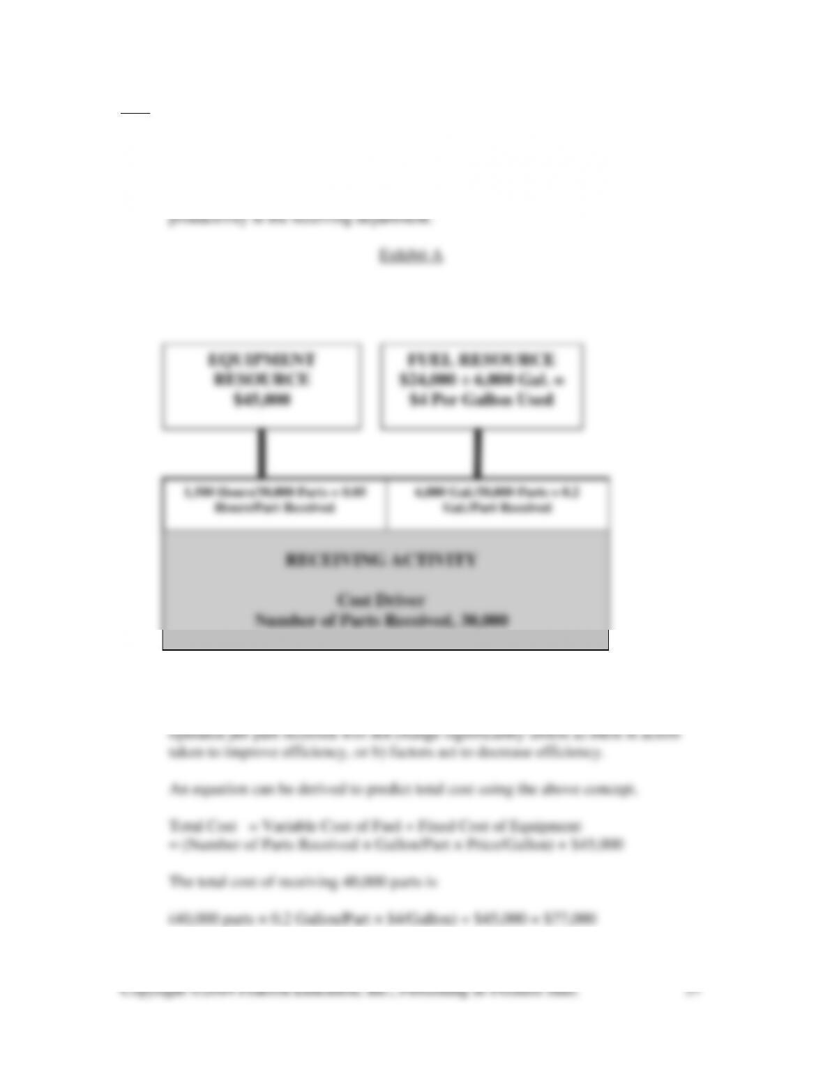
1. Let X = amount of additional fixed costs for advertising
(1,300,000 × £15) +£270,000 -.20(1,300,000 × £15) – (£7,300,000 + X) = 0
2. Let Y = number of seats sold
2-53 (45-55 min.)
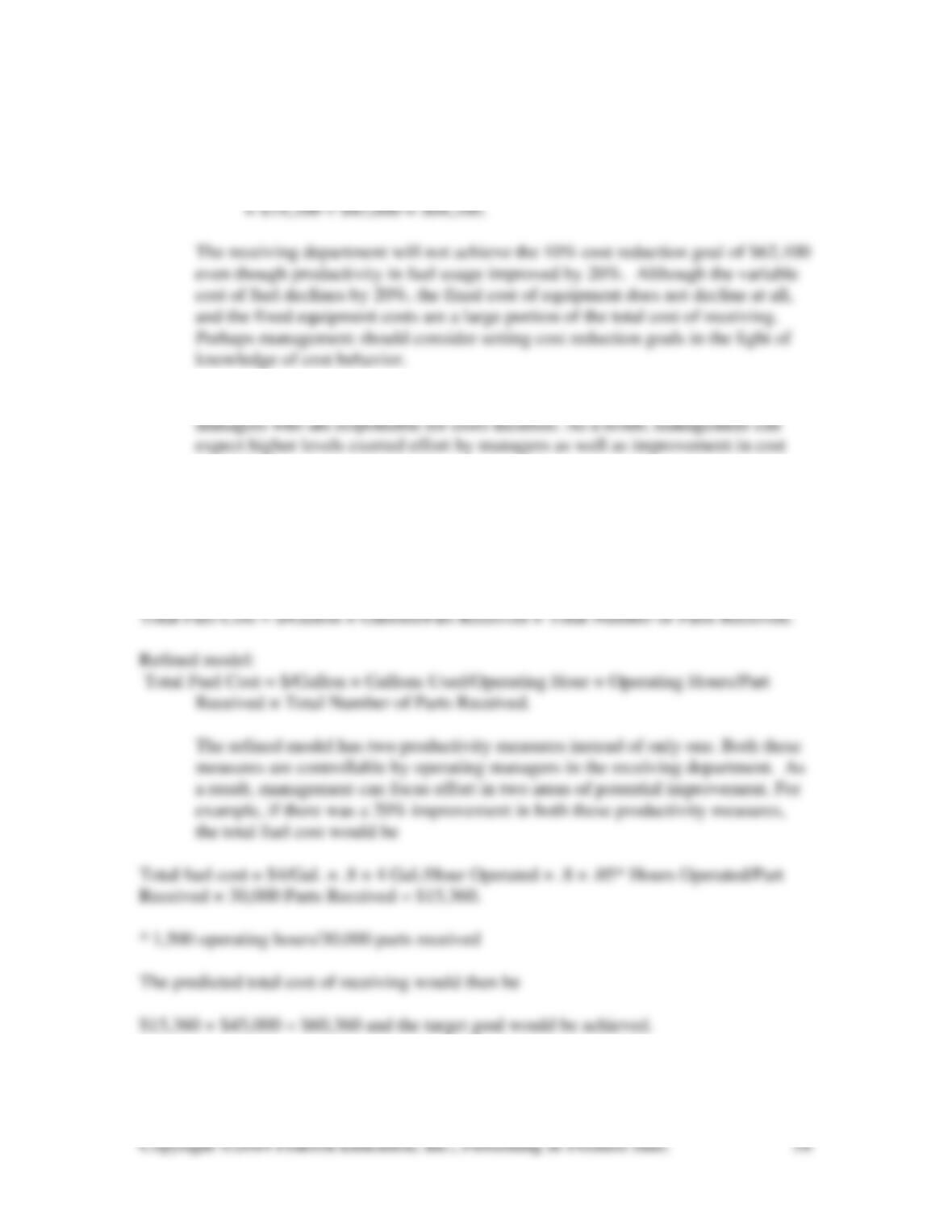
1. Exhibit A shows the relationships between the receiving activity and the resources
used. This information can now be used for cost control purposes. Knowing the
two rates, gallons per part received and machine hours operated per part received,
will help operating managers predict costs. These rates are measures of
2. When the activity level increases, the use of resources will increase. Thus, the
output measures or cost driver levels will increase – that is, total hours and total
gallons. Normally, productivity rates such as gallons per part received and hours
RECEIVING ACTIVITY
Cost Driver
Number of Parts Received, 30,000
EQUIPMENT
RESOURCE
$45,000
FUEL RESOURCE
$24,000 ÷ 6,000 Gal. =
$4 Per Gallon Used
6,000 Gal./30,000 Parts = 0.2
Gal./Part Received
1,500 Hours/30,000 Parts = 0.05
Hours/Part Received
3. The new fuel consumption rate will be .80 × 0.2 gallons/part received = 0.16
gallons per part received. The predicted cost of receiving 30,000 parts is
(30,000 Parts × 0.16 Gallons/Part × $4.00 per Gallon) + $45,000
4. The new model contains productivity measures that are controllable by operating
control.
5. One refinement is to note that total fuel usage is a function of both the efficiency
in machine use as well as efficiency in fuel consumption. In terms of productivity
metrics this can be expressed as follows:
Current model:
2-54 (20-30 min.)
Many shortcuts are available, but this solution uses the equation technique.
1. Let N = meals sold
Sales – Variable expenses – Fixed expenses = Profit before taxes
2. $18N – $9.50N – $17,000 = $0
3. $22N – $11.40N – $25,420 = $8,500
4. Profit = ($22 × 2,550) – ($11.40 × 2,550) – $25,420
Profit = $1,610
5. Profit = ($22 × 2,800) –($11.40 × 2,800) – ($25,420 + $2,300)
Profit = $29,680 – $27,720
2-55 (10-15 min.)
1. The break-even point is $65 fixed cost $2 per day = 32.5 days
3. Let N = 50 days rented.
Under the traditional system the total income is
Revenue – variable cost – fixed cost = $2×N – $0×N – $65
4. Under the traditional system there would be a loss of $53.
5. Blockbuster reduces its risk substantially under the new system because it
reduces its fixed cost.
2-56 (10-15 min.) Amounts are in millions (rounded with slight rounding errors).
Net sales (.9 × $82,559) $74,303
Variable costs:
Cost of goods sold (.9 × $40,768) 36,691
2-57 (15-25 min.)
1. Average revenue per person $8.00 + 4($.50) = $10.00
Total revenue, 200 @ $10.00 = $2,000
2. Number of persons 50 200 350
Total revenue @ $10.00 $ 500 $2,000 $3,500
Fixed costs
3. Number of persons 50 200 350
Revenue $ 500 $2,000 $3,500
Variable costs 50 200 350
Contribution margin $ 450 $1,800 $3,150
2-58 (10-20 min.)
1. To compute eBay’s operating income, we need to know fixed and variable costs. We
are given that its fixed costs are $37 million. Variable costs in the first quarter of 2001
were:
Operating expenses – Fixed costs = Variable costs
$123 million – $37 million = $86 million
2. When sales increased 59%, operating income increased by 130%. This is an example
of the effect of operating leverage. The variable cost percentage is approximately $86 ÷
$154 = 56%. Thus, the contribution margin percentage is 100% – 56% = 44%. Every