Copyright ©2014 Pearson Education, Inc., Publishing as Prentice Hall.
577
13-50 (15-20 min.)
(Note that final dollar amounts are rounded to the nearest dollar.)
1. Overhead rate = ($277,800 + $103,200) ÷ 69,450 machine hours
= $5.48596 per machine hour
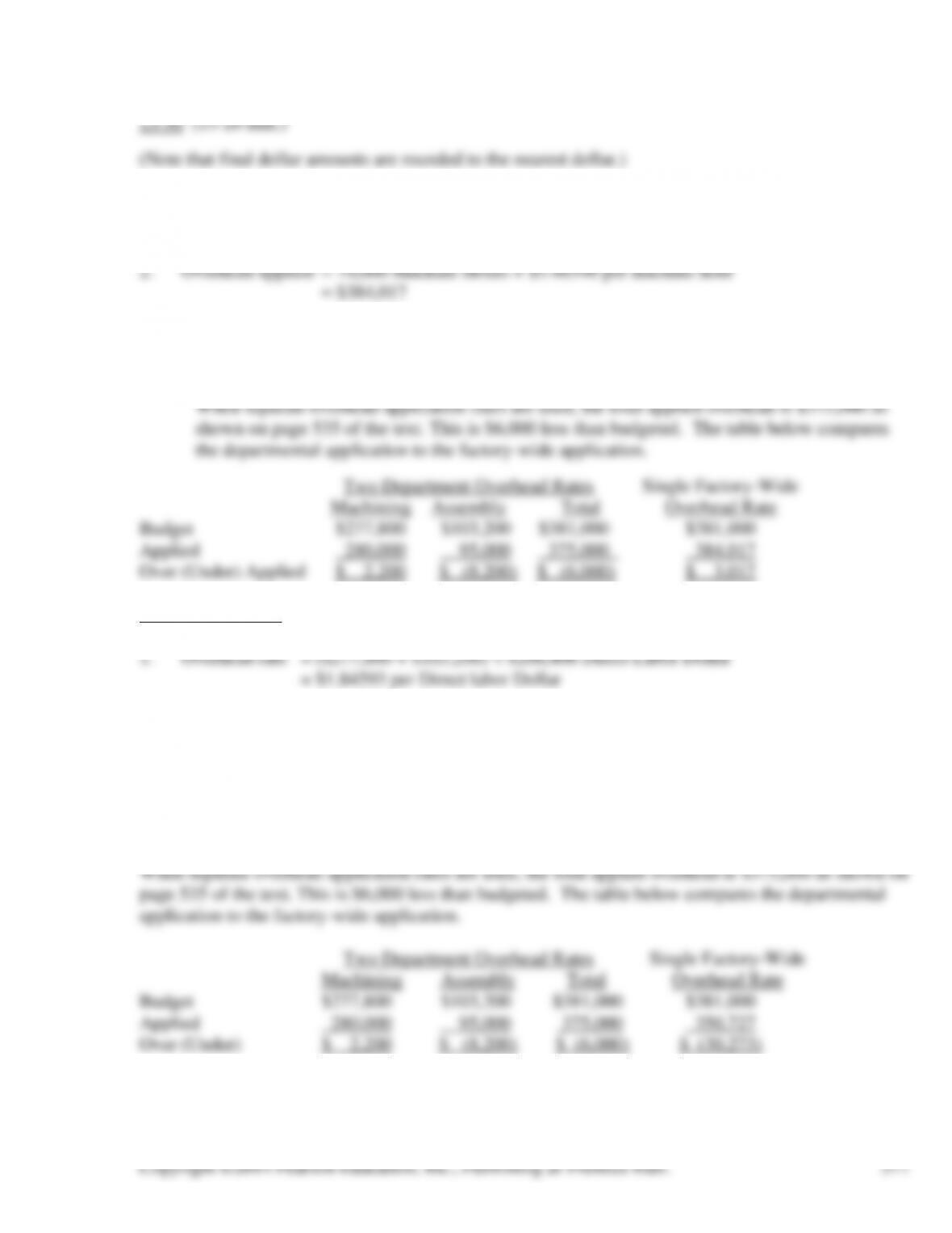
3. The overhead is overapplied by $384,017 – $381,000 = $3,017. This is because the amount of
machine hours used exceeds the budgeted amount by 70,000 – 69,450 = 550 and 550 ×
$5.48596 = $3,017.
13-51 (15-20 min.) (Note that final dollar amounts are rounded to the nearest dollar.)
2. Overhead applied = $190,000 Direct Labor Dollars × $1.84593
= $350,727
3. The overhead is underapplied by $381,000 – $350,727 = $30,273. This is because the direct labor
cost is less than the budgeted amount by $206,400 – $190,000 = $16,400 and $16,400 × $1.84593 =
$30,273.
Copyright ©2014 Pearson Education, Inc., Publishing as Prentice Hall.
578
13-52 (20-35 min.)
1. $10,000,000 ÷ $5,000,000 = 200% of direct labor
2. ($10,000,000 – $3,000,000) ÷ $5,000,000 = 140% of direct labor
3. Engagement
Eagledale First Valley
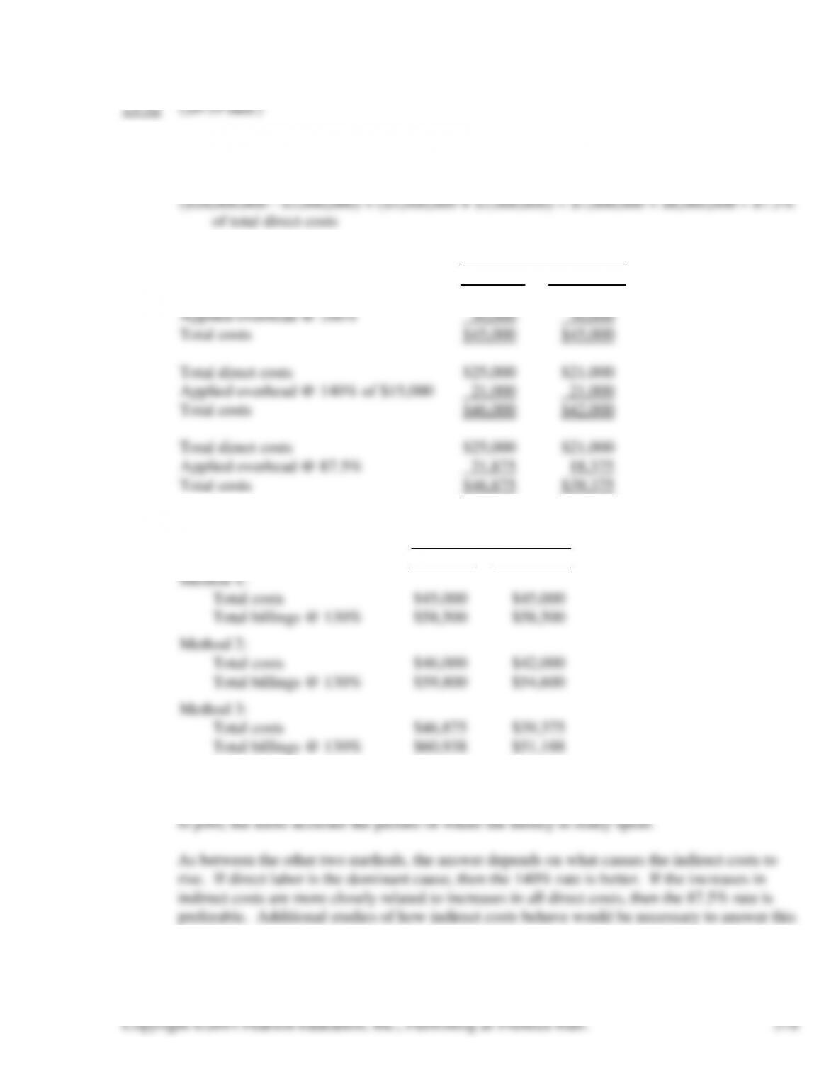
Direct labor $15,000 $15,000
4. The billings would differ significantly:
Engagement
Eagledale First Valley
5. The first method is inferior to the other two because the latter give more accurate measures of
how specific jobs cause increases in costs. In general, the more costs that are directly charged
question.
Copyright ©2014 Pearson Education, Inc., Publishing as Prentice Hall.
579
13-53 (15 min.)
1. If other departments are indeed providing services to the water and sewer department, it is
certainly appropriate to include the cost of these services in the water and sewer department’s
2. It would be useful to identify the activities involved when other departments provide services
to the water and sewer department. If it is not too expensive, it would be worthwhile to
13-54 (15-25 min.) This problem is intended to highlight the distinction and relation between
accounting for control and accounting for product costing.
1. First six months:
2. Overhead rate:
Fixed, $350,000 ÷ 100,000 DLH $3.50 per DLH
Variable, $150,000 ÷ 100,000 DLH 1.50 per DLH
8,000. Fixed overhead was thus underapplied by 8,000 × $3.50 = $28,000. Actual
Copyright ©2014 Pearson Education, Inc., Publishing as Prentice Hall.
580
13-55 (35-45 min.) This is an excellent problem for presentation in class. It is less satisfactory as a
homework assignment because students tend to make the problem harder than it really is.
1. One way to present the problem in class is to begin with 9 columns on the board or screen.
Each column lists the sales and production quantities. Provide six rows for the variable–
costing statement and seven rows for the absorption-costing statement, labeled as in the
format provided in the problem, there are 18 “income statements” to be completed. Ask a
different student to complete each statement. Patterns soon become clear, and students fill in
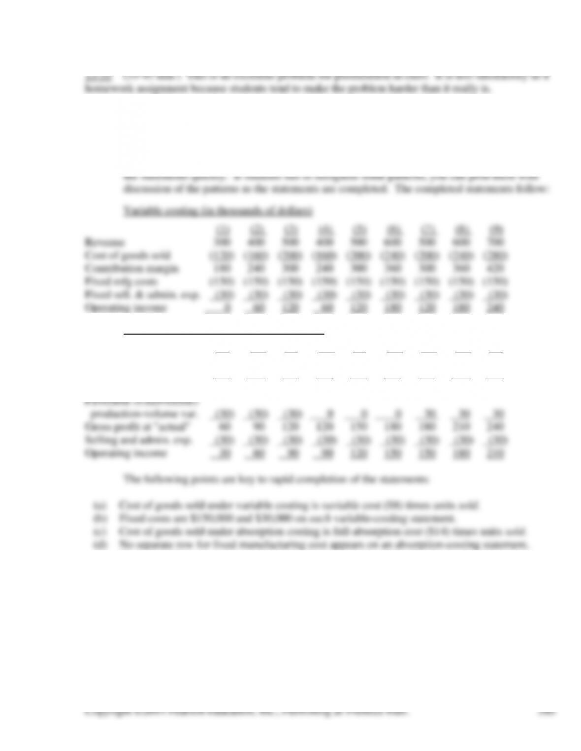
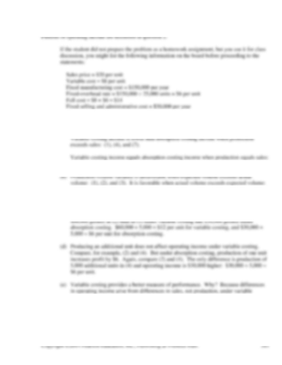
Absorption costing (in thousands of dollars)
(1) (2) (3) (4) (5) (6) (7) (8) (9)
Revenue 300 400 500 400 500 600 500 600 700
Cost of goods sold (210) (280) (350) (280) (350) (420) (350) (420) (490)
Gross profit at standard 90 120 150 120 150 180 150 180 210
Fixed manufacturing costs are included in cost of goods sold and in the production-volume
variance.
(e) Production-volume variance is production units less expected unit volume times fixed
manufacturing cost per unit ($6).
(f) Selling and administrative expenses are not inventoried; even on an absorption-costing
statement the $30,000 is charged each period.
Copyright ©2014 Pearson Education, Inc., Publishing as Prentice Hall.
581
Patterns of operating income are discussed in question 2.
If the student did not prepare the problem as a homework assignment, but you use it for class
discussion, you might list the following information on the board before proceeding to the
statements:
Sales price = $20 per unit
Variable cost = $8 per unit
Fixed manufacturing cost = $150,000 per year
Fixed-overhead rate = $150,000 ÷ 25,000 units = $6 per unit
Full cost = $8 + $6 = $14
Fixed selling and administrative cost = $30,000 per year
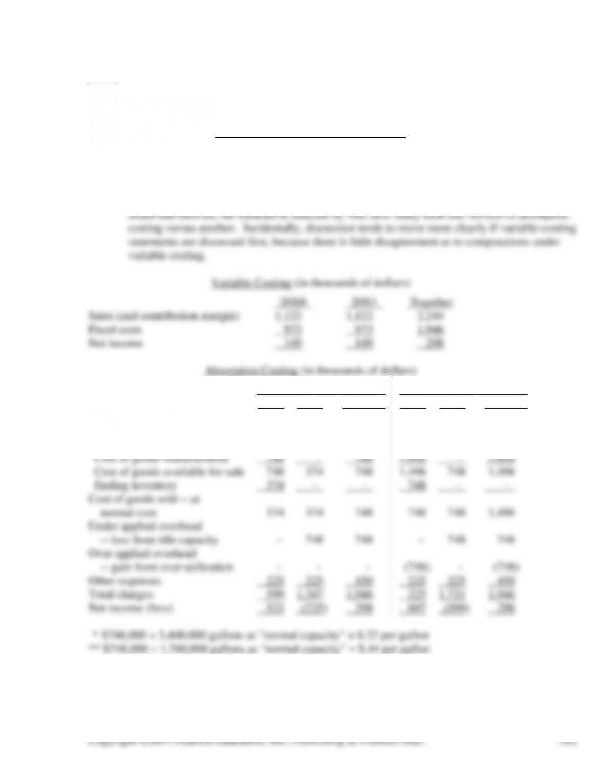
2. (a) Variable-costing income is greater than absorption-costing income when sales exceed
production: (3), (6), and (9).
(2), (5), and (8).
(7), (8), and (9).
(c) Each additional unit sold adds $20 – $8 = $12 to profit under variable costing and $20 –
$14 = $6 under absorption costing. For example, compare (1) and (2). Production is
20,000 units in each case, but sales are 5,000 units greater in (2). Operating income is
costing.
13-56 (25-35 min.)
Please allow ample time for classroom discussion.
1. Comments on the Following Statements
The accounting for fixed overhead in absorption costing is affected primarily by what
expected production volume is selected as a base (the denominator) for applying fixed
overhead to product. In this case, is 1,700,000 gallons per year, 3,400,000 gallons, or some
other activity level the most appropriate base? We usually place the above possibilities on the
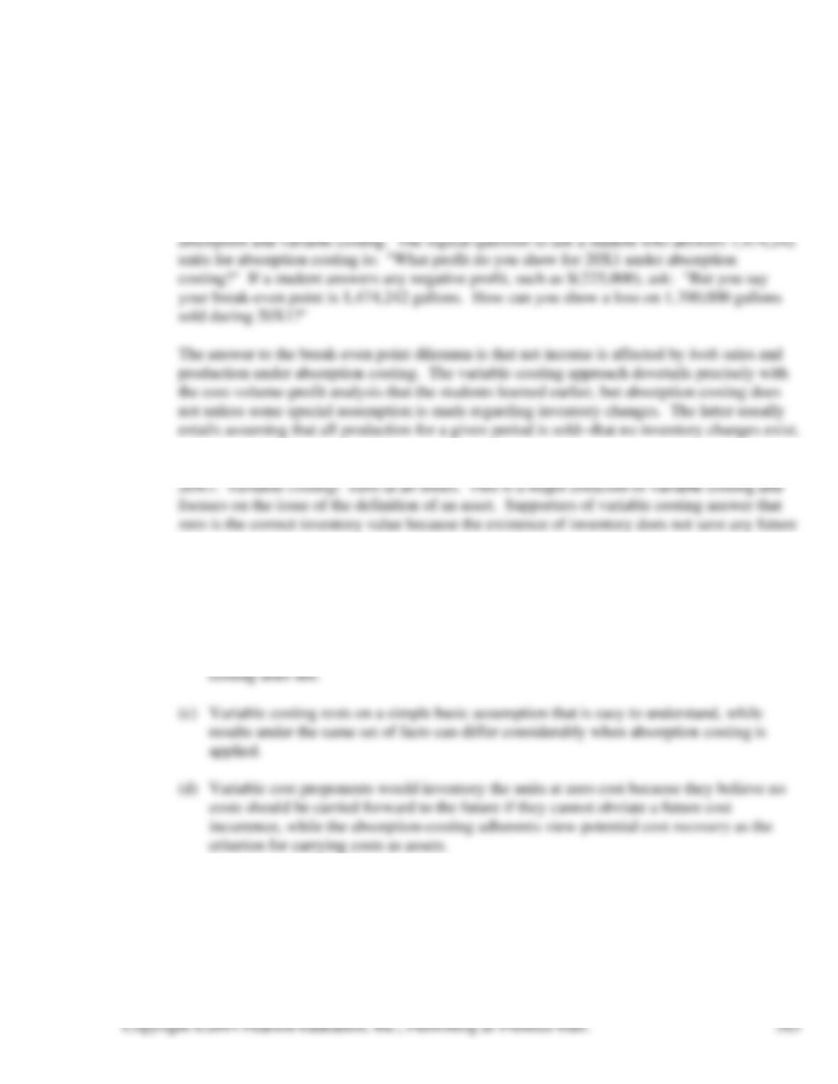
Option One* Option Two**
20X0 20X1 Together 20X0 20X1 Together
Sales 1,122 1,122 2,244 1,122 1,122 2,244
Less cost of goods sold:
Beginning inventory – 374 – – 748 –
2. Break-even point = Fixed expenses ÷ Contribution margin per gallon
= $973,000 ÷ $.66 = 1,474,242 gallons
If the company would sell 225,758 fewer gallons per year at $.66 each, it would just break
even.
Most students will say that the break-even point is 1,474,242 gallons per year under both
3. Absorption costing: Either $374,000 or $748,000 at the end of 20X0 and zero at the end of
cost.
4. Comments should include the following:
(a) The central issue is the timing of release of fixed factory overhead to expense.
(b) Variable costing dovetails exactly with general break-even analysis, while absorption
Copyright ©2014 Pearson Education, Inc., Publishing as Prentice Hall.
584
13-57 (25-30 min.)
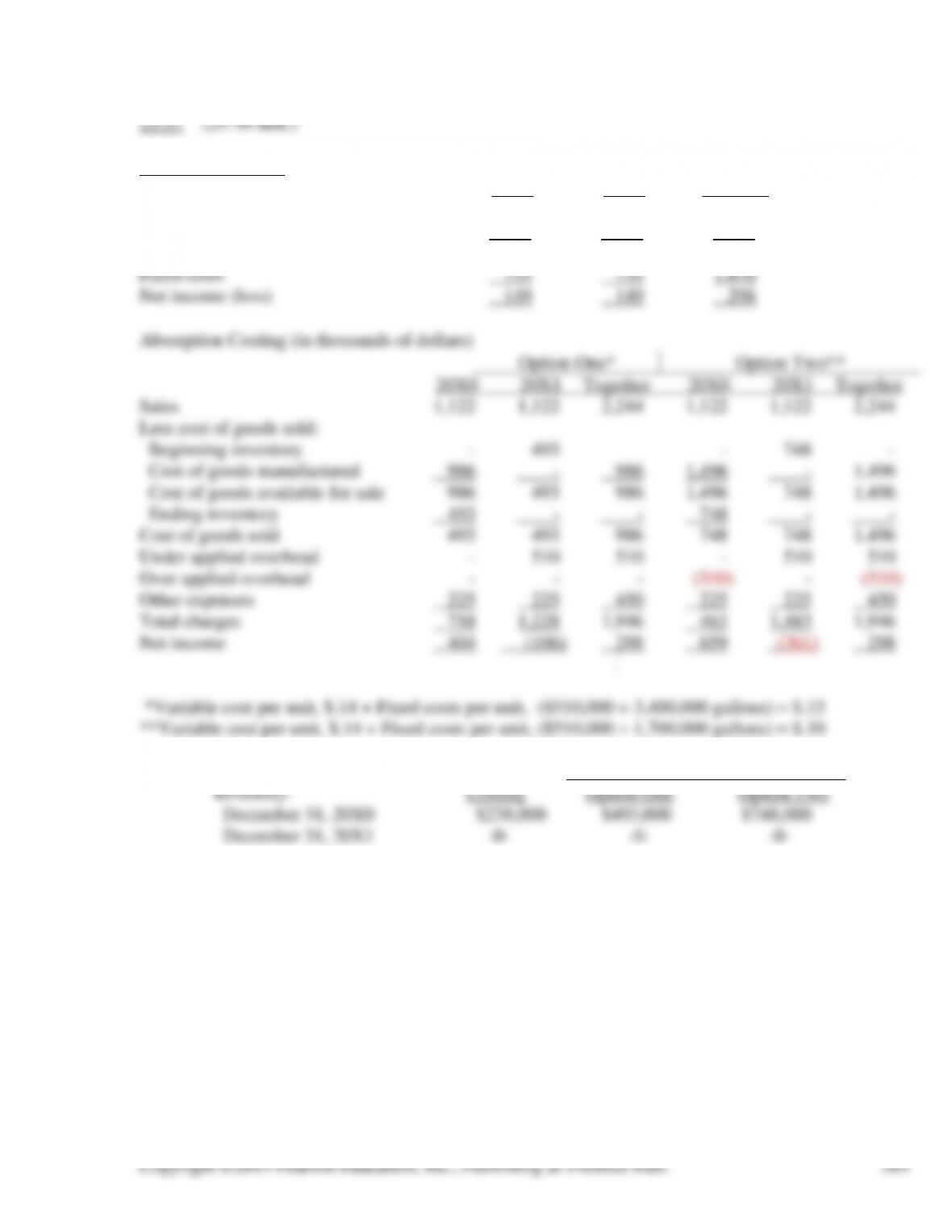
1. Variable Costing (in thousands of dollars)
20X0 20X1 Together
Sales 1,122 1,122 2,244
Variable cost of sales @ $.14 per gallon 238 238 476
Contribution margin 884 884 1,768
Absorption Costing (in thousands of dollars)
Option One*
Option Two**
20X0 20X1 Together 20X0 20X1 Together
Sales 1,122 1,122 2,244 1,122 1,122 2,244
Less cost of goods sold:
Beginning inventory – 493 – 748 –
Cost of goods manufactured 986 – 986 1,496 – 1,496
Cost of goods available for sale 986 493 986 1,496 748 1,496
Ending inventory 493 – – 748 – –
Cost of goods sold 493 493 986 748 748 1,496
Under applied overhead – 510 510 – 510 510
Over applied overhead – – – (510) – (510)
Other expenses 225 225 450 225 225 450
Total charges 718 1,228 1,946 463 1,483 1,946
Net income 404 (106) 298 659 (361) 298
*Variable cost per unit, $.14 + Fixed costs per unit, ($510,000 ÷ 3,400,000 gallons) = $.15
**Variable cost per unit, $.14 + Fixed costs per unit, ($510,000 ÷ 1,700,000 gallons) = $.30
2. Variable Absorption Costing
13-58 (30-35 min.)
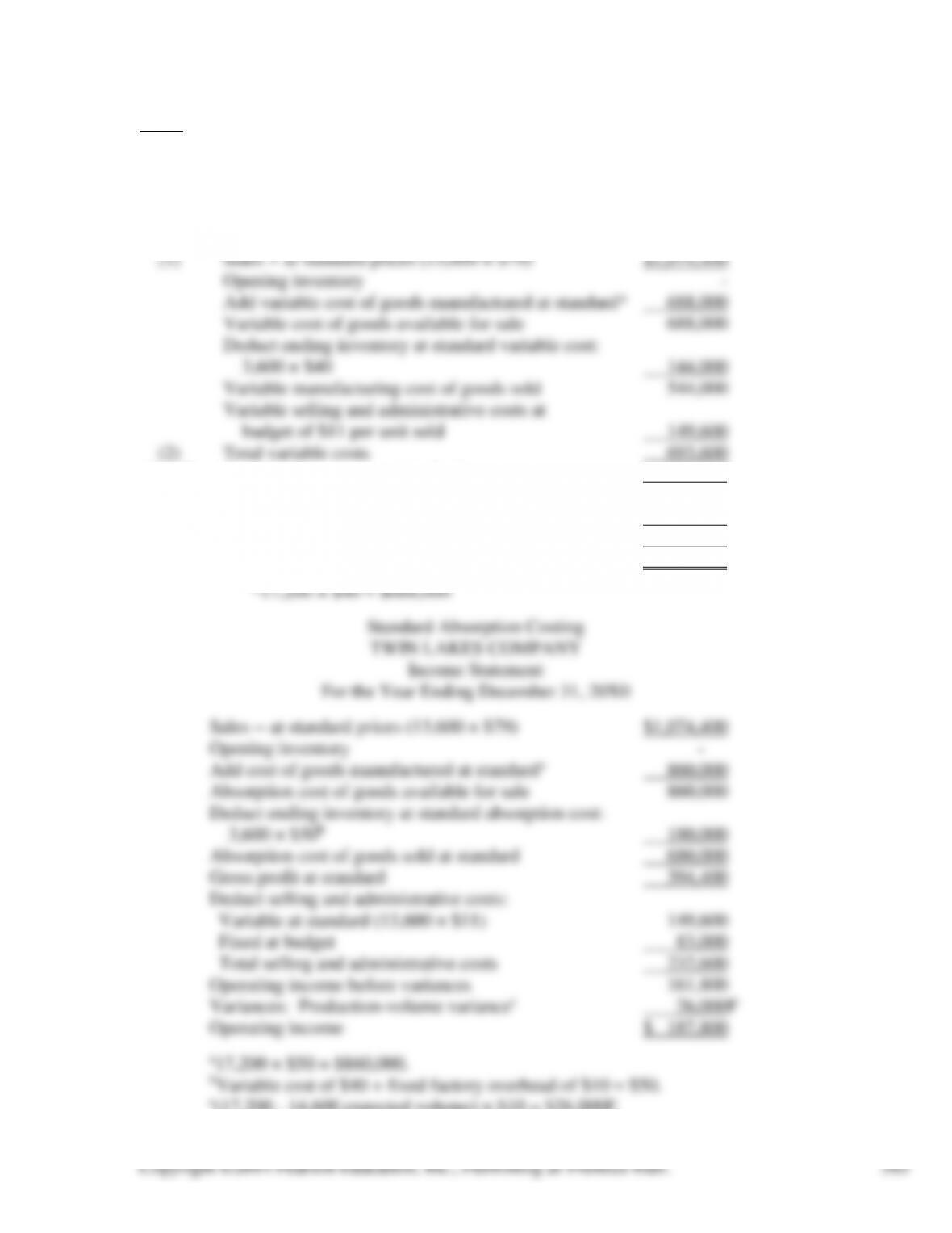
1. Standard Variable Costing
TWIN LAKES COMPANY
Income Statement
For the Year Ended December 31, 20X0
(1) – (2) Contribution margin at standard 380,800
Fixed factory overhead at budget 146,000
Fixed selling and administrative costs 83,000
Total fixed costs 229,000
Operating income $ 151,800
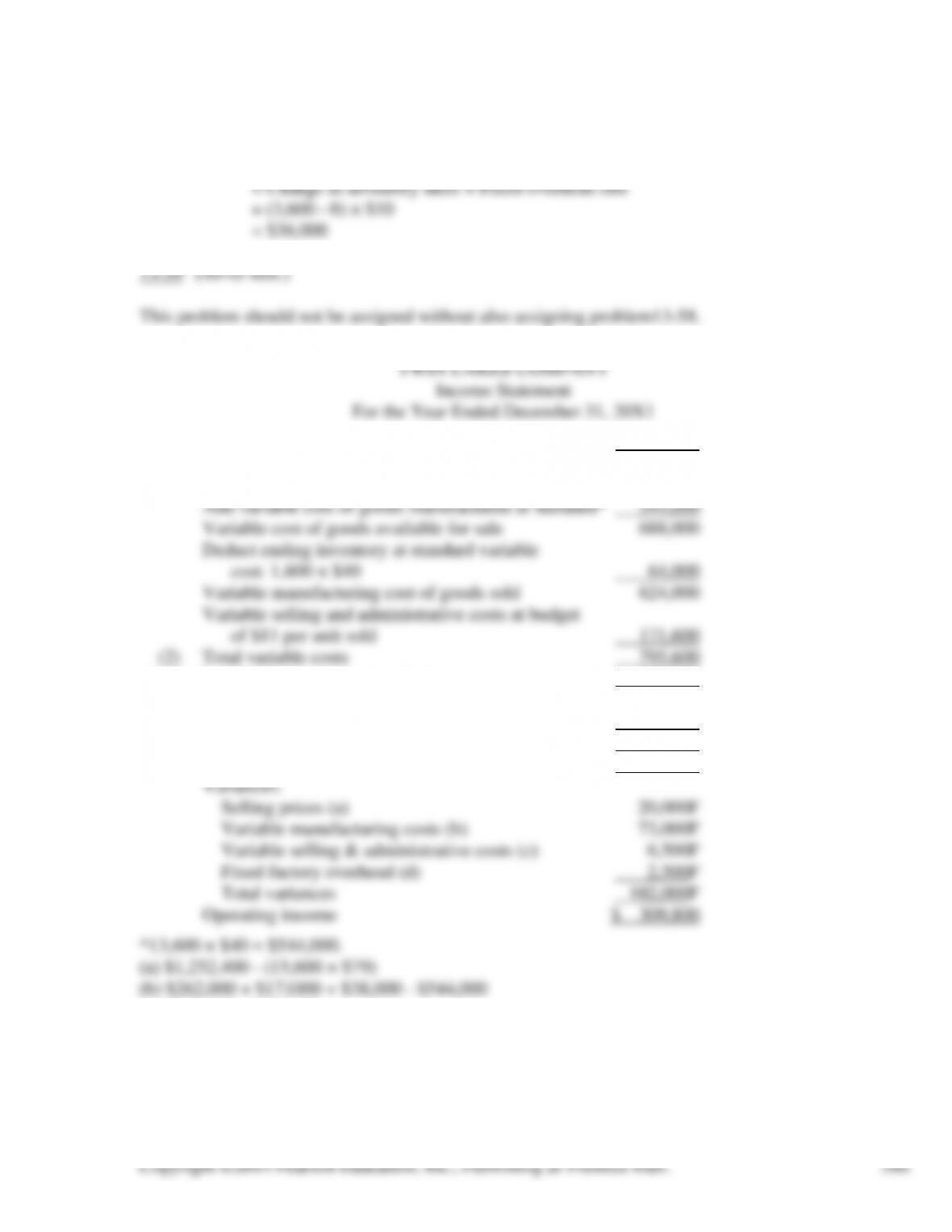
2. If inventories increase, operating income will be higher under absorption costing:
Difference in operating income
1. Standard Variable Costing
(1) Sales — at standard prices (15,600 × $79) $1,232,400
Opening inventory, at standard variable
cost: 3,600 × $40 144,000
(1)-(2) Contribution margin at standard 436,800
Fixed factory overhead at budget 146,000
Fixed selling and administrative costs 83,000
Total fixed costs 229,000
Operating income before variances 207,800
(c) $165,100 – $171,600
(d) $143,500 – $146,000
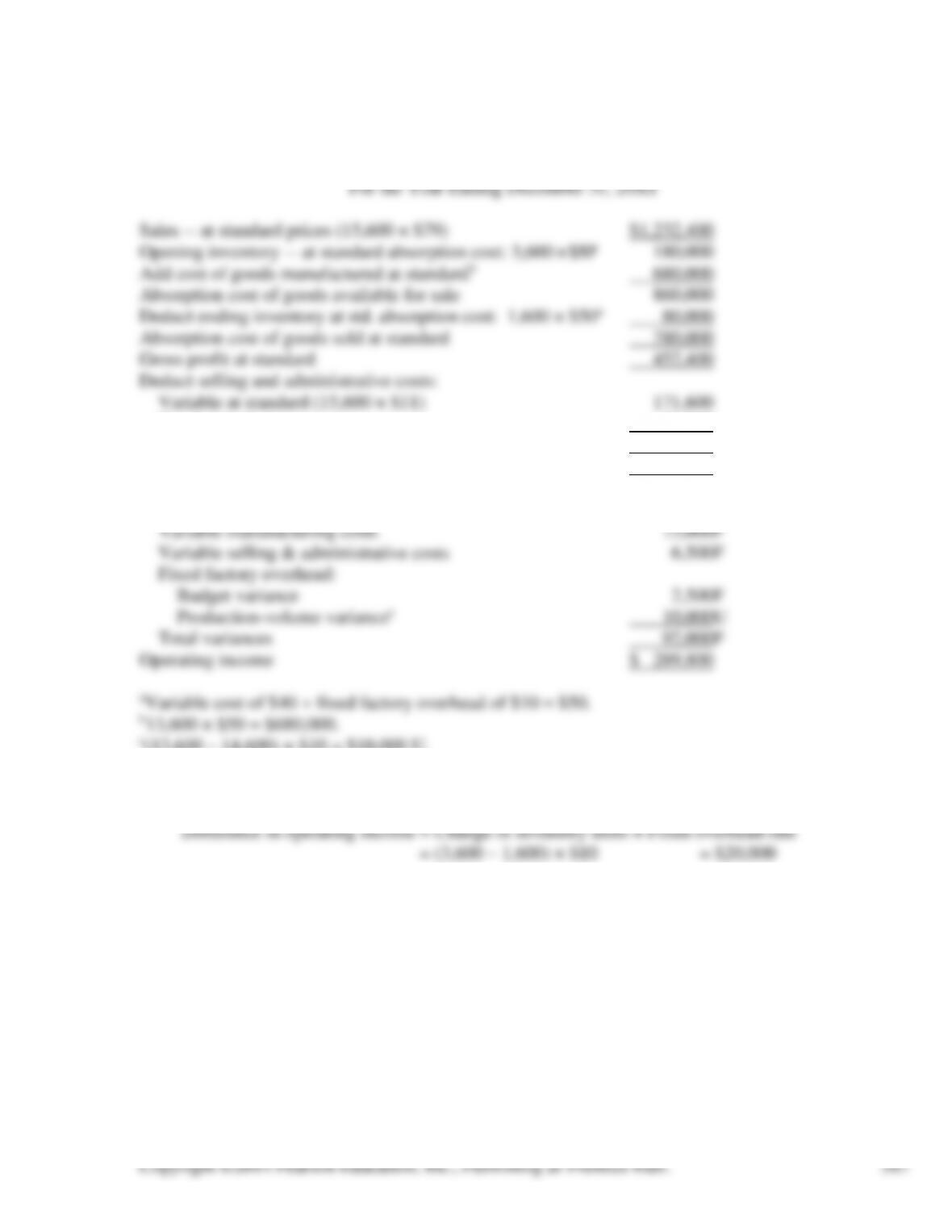
Standard Absorption Costing
TWIN LAKES COMPANY
Income Statement
Fixed at budget 83,000
Total selling and administrative costs 254,600
Operating income before variances 197,800
Variances:
Selling prices 20,000F
2. If inventories decrease, operating income is lower under absorption costing:
13-60 (30-40 min.) This is a straightforward problem that is quite informative for most students.
1. $60,000 ÷ 7,500 hrs. = $8.00 per hour;
$8.00 × 2 hours = $16.00 per unit
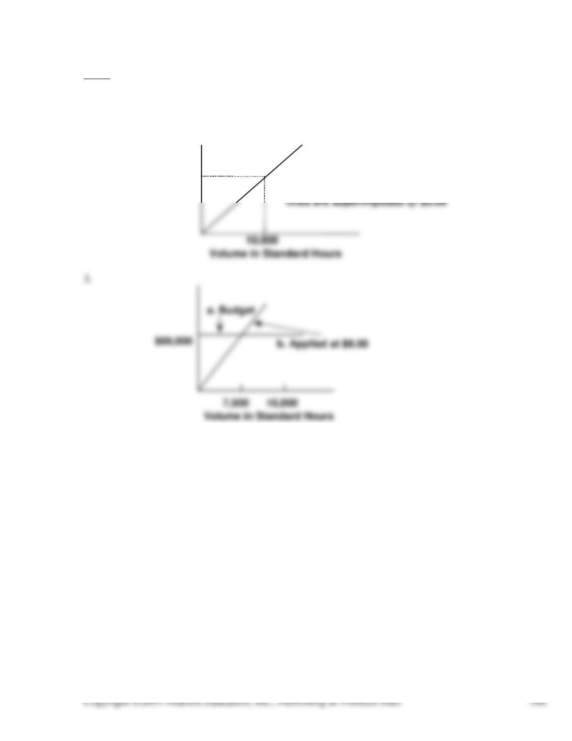
2.
Volume in Standard Hours
$50,000
a & b. Budgeted and applied
lines are superimposed @ $5.00
10,000
3.
$60,000
b. Applied at $8.00
Volume in Standard Hours
10,000
7,500
a. Budget
Copyright ©2014 Pearson Education, Inc., Publishing as Prentice Hall.
589
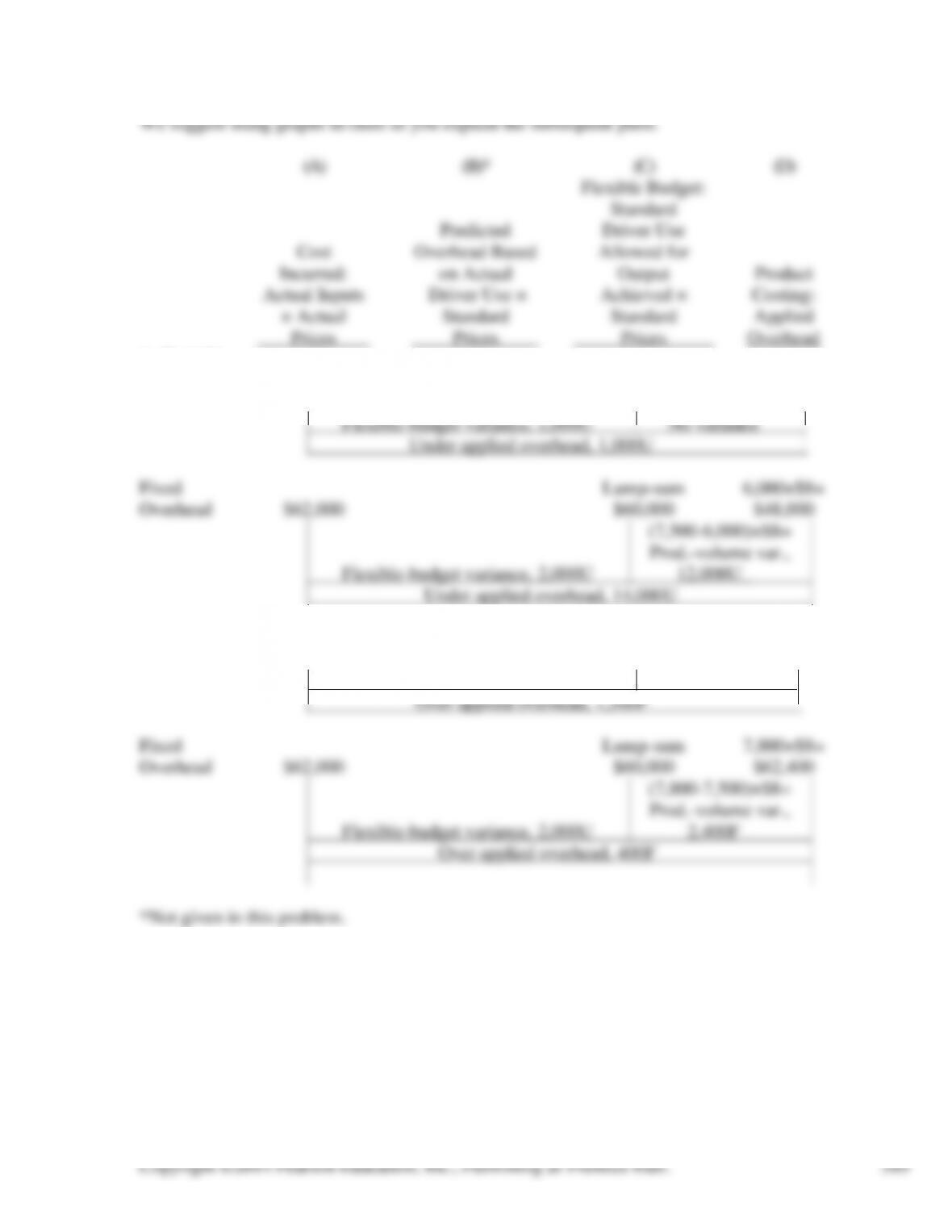
We suggest using graphs in class as you explain the subsequent parts.
(A) (B)* (C) (D)
Flexible Budget:
Standard
Predicted Driver Use
Cost Overhead Based Allowed for
Incurred: on Actual Output Product
Actual Inputs Driver Use × Achieved × Costing:
× Actual Standard Standard Applied
Prices Prices Prices Overhead
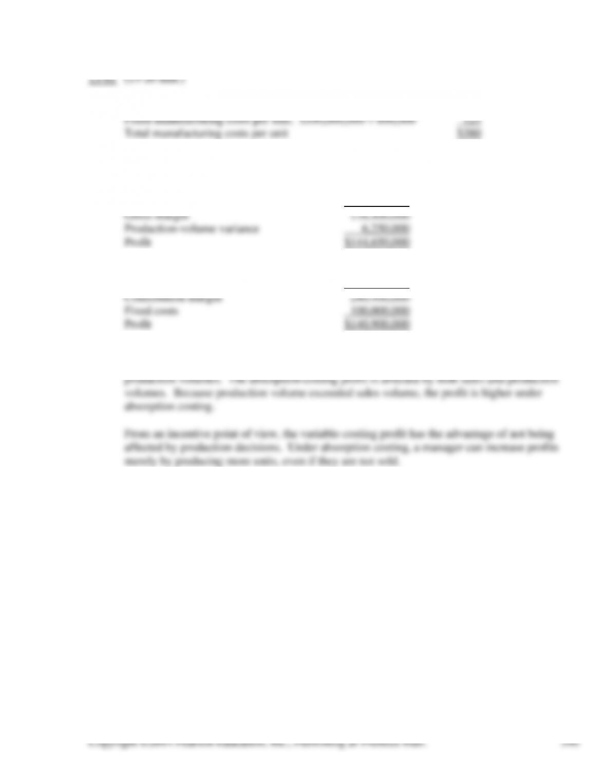
4. Variable
6,000×$5=
Overhead $31,000 $30,000 $30,000
5. Variable 7,800×$5=
Overhead $37,700 $39,000 $39,000
Flexible-budget variance, 1,300F No variance
Copyright ©2014 Pearson Education, Inc., Publishing as Prentice Hall.
590
13-61 (15-20 min.)
1. Variable manufacturing costs per unit, $204,000,000 ÷ 800,000 $255
2. Production-volume variance = (800,000 – 850,000) × $125 = $6,250,000 F
3. Revenue (820,000 × $548.78) $450,000,000
Cost of goods sold (820,000 × $380) 311,600,000
4. Revenue (820,000 × $548.78) $450,000,000
Cost of goods sold (820,000 × $255) 209,100,000
5. Neither measure is inherently better. They give different signals about performance. The
variable-costing profit is a better measure of the effect of sales on profit. It is not affected by
13-62 (10 min.)
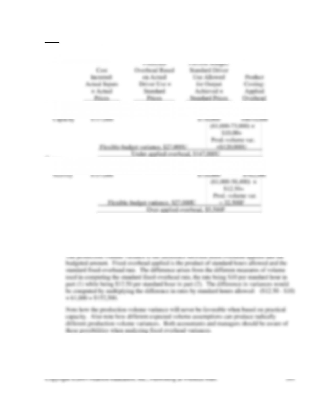
Overhead rates: $730,000 ÷ 58,400 = $12.50 and $730,000 ÷ 73,000 = $10.00.
1. Using
Practical 61,000×$10
2. Using
Expected 61,000×$12.50=
3. The flexible-budget variance for fixed overhead is the difference between the amount incurred
and the budget figure. The budget figure is the same regardless of the actual level of activity
and the rate used in applying fixed overhead. Consequently the flexible-budget variances in
parts (1) and (2) would be identical.