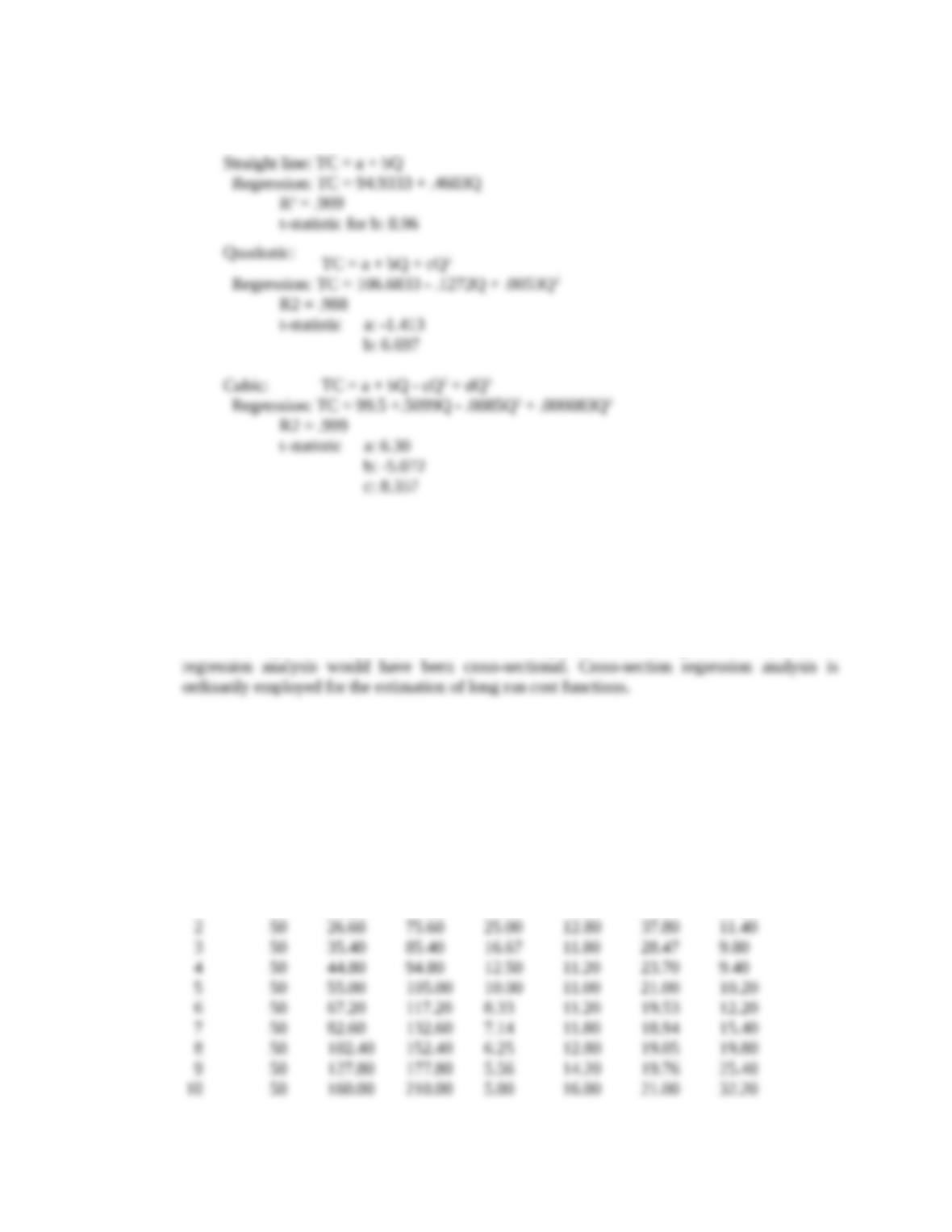
b.-c. The following three formulas were used:
The cubic function appears to give the best fit; it has the highest coefficient of determination,
and all the t-statistics are significant. The signs of the coefficients (all positive except the
coefficient of Q2) are correct.
d. Yes. Time series analysis is usually employed for short-run cost studies.
e. If the data represented observations for 10 different plants at the same point in time, then the
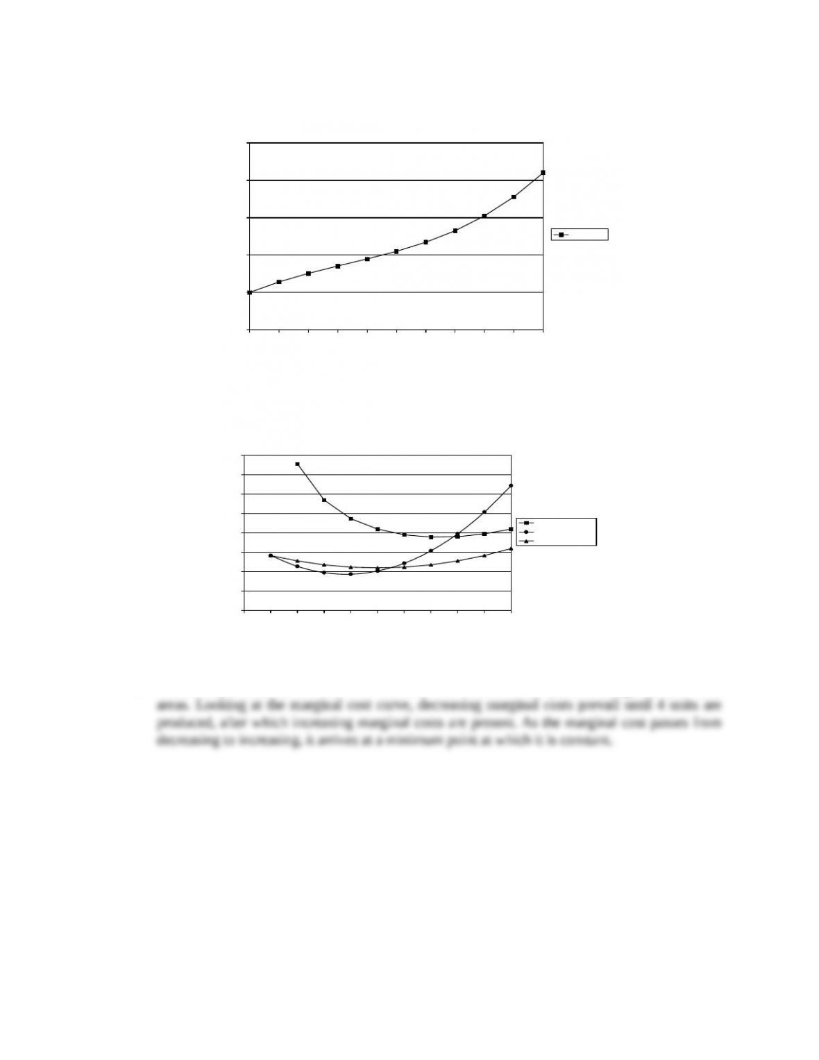
10. The following table represents all the relevant cost data for quantities 1 to 10. It has been assumed
that the constant term in the equation (equaling 50) represents fixed cost. Marginal costs have been
calculated as the differences in total cost as one unit of quantity is added (rather than using calculus.
The interested student can make this calculation).
Quantity
Total
Fixed
Cost
Total
Variable
Cost
Average
Total
Cost
Average
Fixed
Cost
Variable
Cost
Total
Cost
Margina
l Cost
0 50 0.00 50.00
1 50 14.20 64.20 50.00 14.20 64.20 14.20
a.
Figure 7.6
b. All data are shown in the table above.
Figure 7.7
c. Grand Corporation has a cubic cost function. This means that it passes through all three cost
0
50
100
150
200
250
0 1 2 3 4 5 6 7 8 9 10
Q
Total Cost
TC ($)
0
5
10
15
20
25
30
35
40
0 1 2 3 4 5 6 7 8 9 10
Q
A v e ra g e C o st
M arg in a l C o s t
A v e ra g e Var C o s t
$
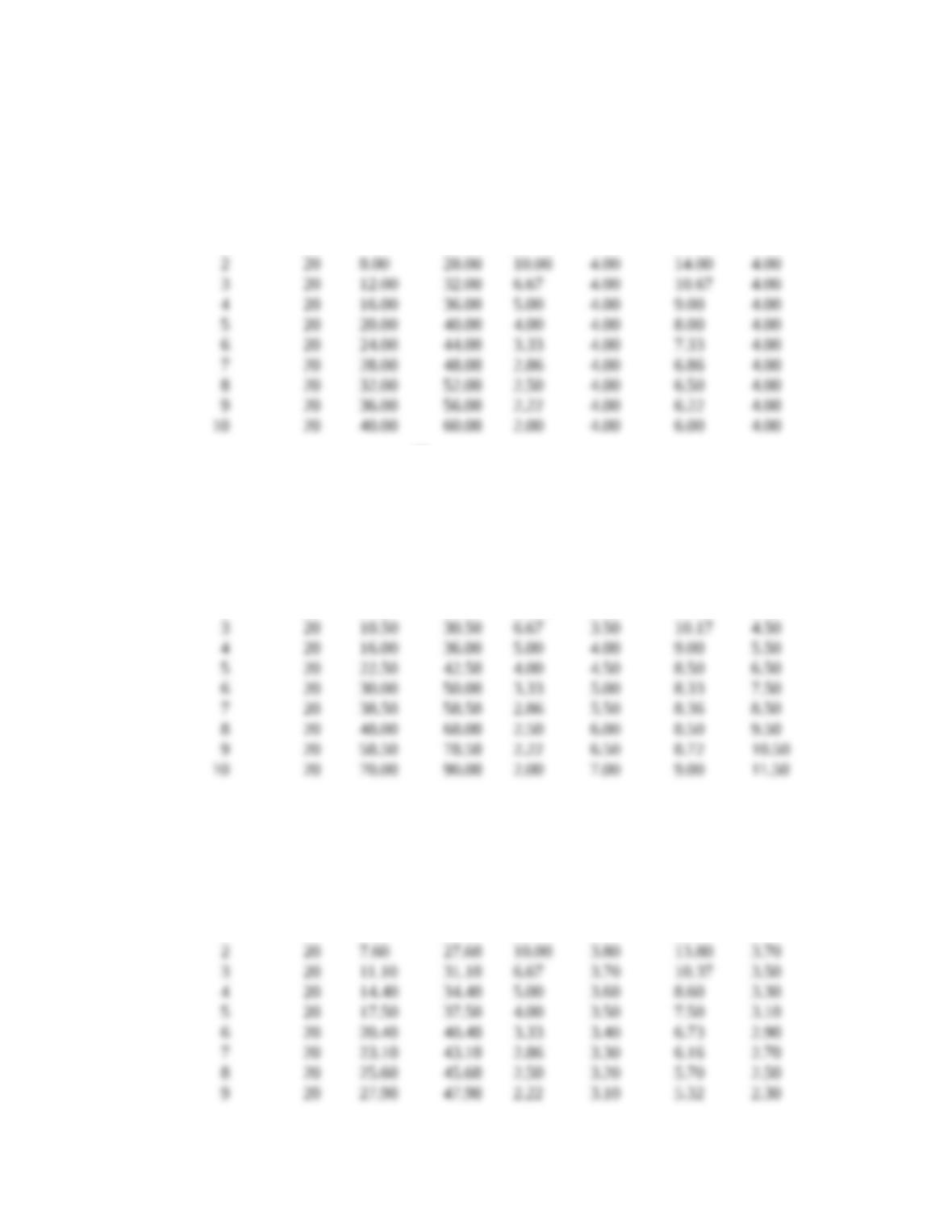
11. a. (1) TC = 20 + 4Q
Quantity
Total
Fixed
Cost
Total
Variable
Cost
Total
Cost
Average
Fixed
Cost
Average
Variable
Cost
Average
Total
Cost
Marginal Cost
0 20 0.00 20.00
1 20 4.00 24.00 20.00 4.00 24.00 4.00
(2) TC = 20 + 2Q + .5Q2
Quantity
Total
Fixed
Cost
Total
Variable
Cost
Total
Cost
Average
Fixed
Cost
Average
Variable
Cost
Average
Total
Cost
Marginal Cost
0 20 0.00 20.00
1 20 2.50 22.50 20.00 2.50 22.50 2.50
2 20 6.00 26.00 10.00 3.00 13.00 3.50
(3) TC = 20 + 4Q -.1Q2
Quantity
Total
Fixed
Cost
Total
Variable
Cost
Total
Cost
Average
Fixed
Cost
Average
Variable
Cost
Average
Total
Cost
Marginal Cost
0 20 0.00 20.00
1 20 3.90 23.90 20.00 3.90 23.90 3.90
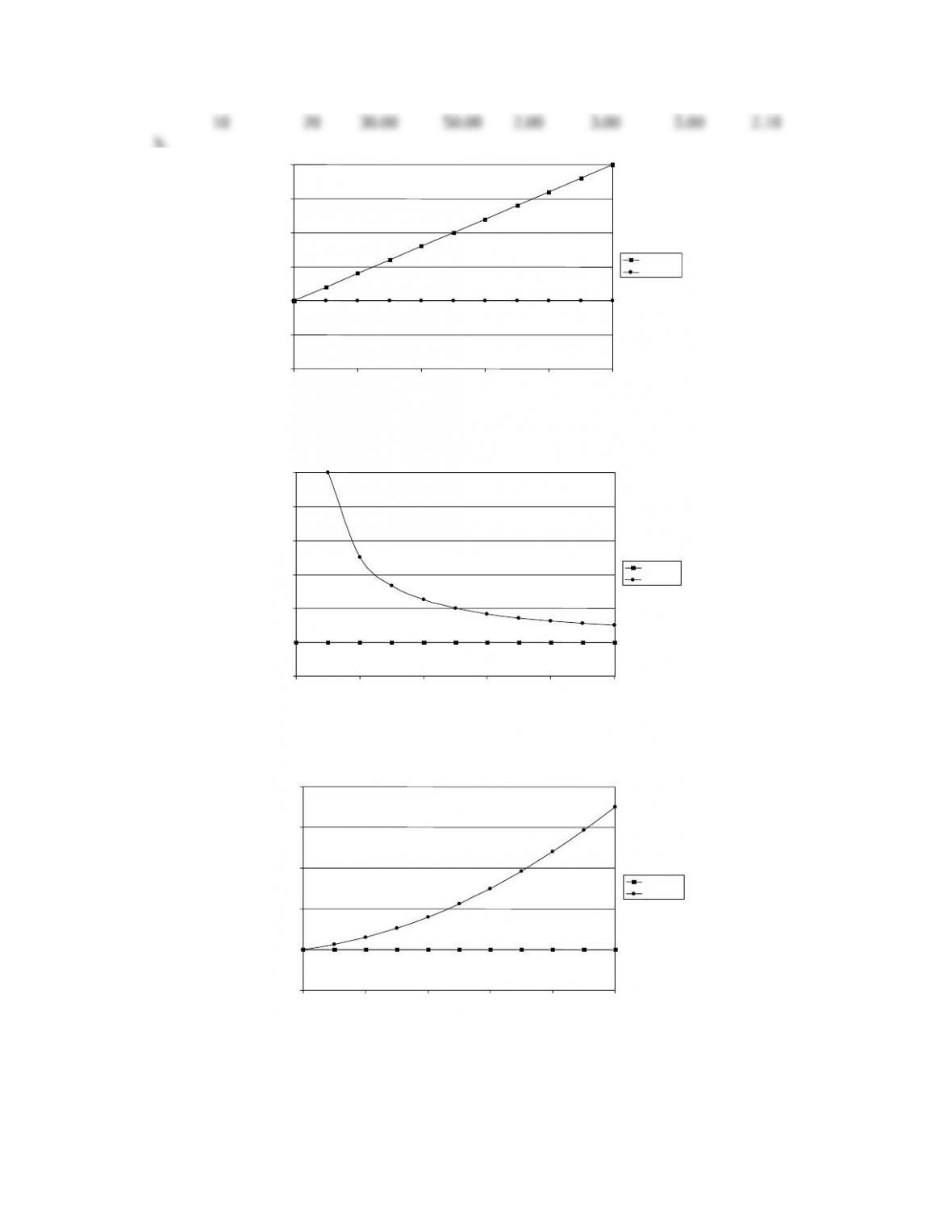
b.
Figure 7.8
Figure 7.9
Figure 7.10
0
10
20
30
40
50
60
0246810
Q
Total Cost
Fixed Cost
$
0
4
8
12
16
20
24
0 2 4 6 8 10
Q
AVC = MC
Av Cost
$
0
20
40
60
80
100
0 2 4 6 8 10
Q
Fixed Cost
Total Cost
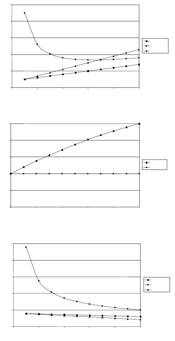
Figure 7.11
Figure 7.12
Figure 7.13
0
5
10
15
20
25
0 2 4 6 8 10
Q
Av Var Cost
Av Cost
Marg Cost
0
5
10
15
20
25
0246810
Q
Av Var Cost
Av Cost
Marg Cost
0
10
20
30
40
50
0246810
Q
Total Cost
Fixed Cost
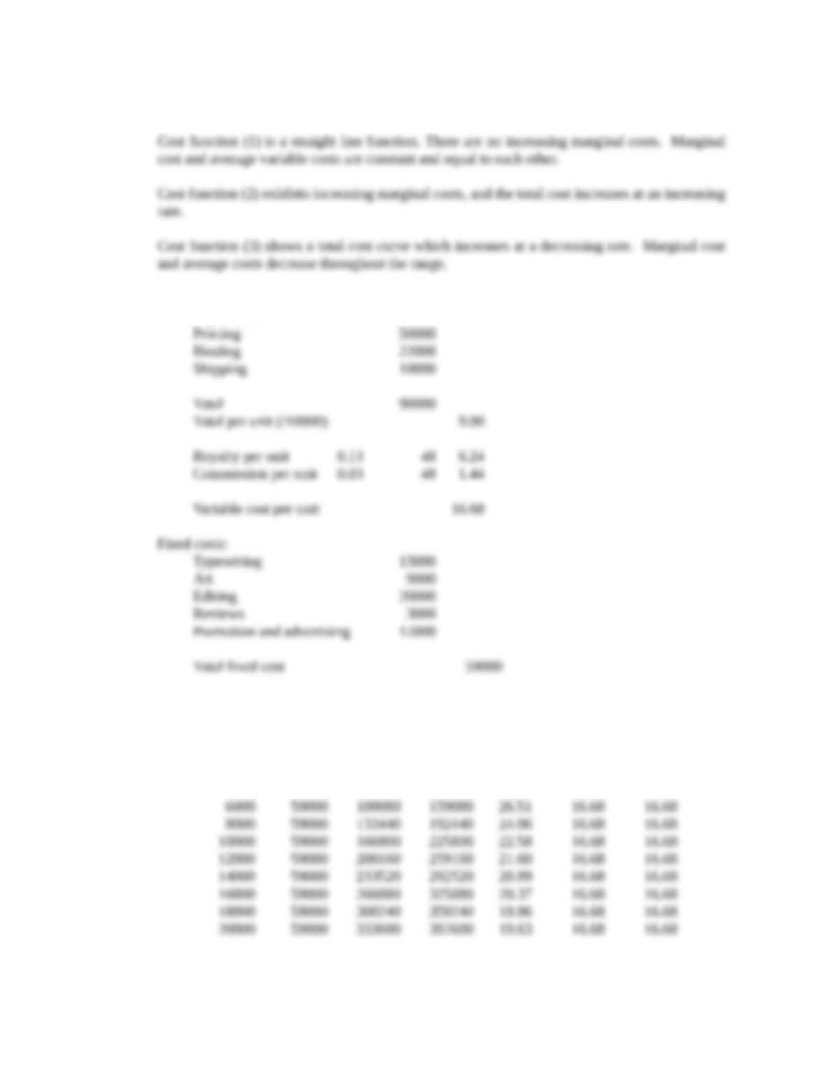
c. We have assumed that the first term on the right side of the equation (20) represents fixed costs.
12. a. Variable costs:
Paper stock 8000
Quantity Fixed
Cost
Variable
Cost
Total
Cost
Average
Total
Cost
Average
Variable
Cost
Marginal Cost
0 59000 0 59000
2000 59000 33360 92360 46.18 16.68 16.68
4000 59000 66720 125720 31.43 16.68 16.68
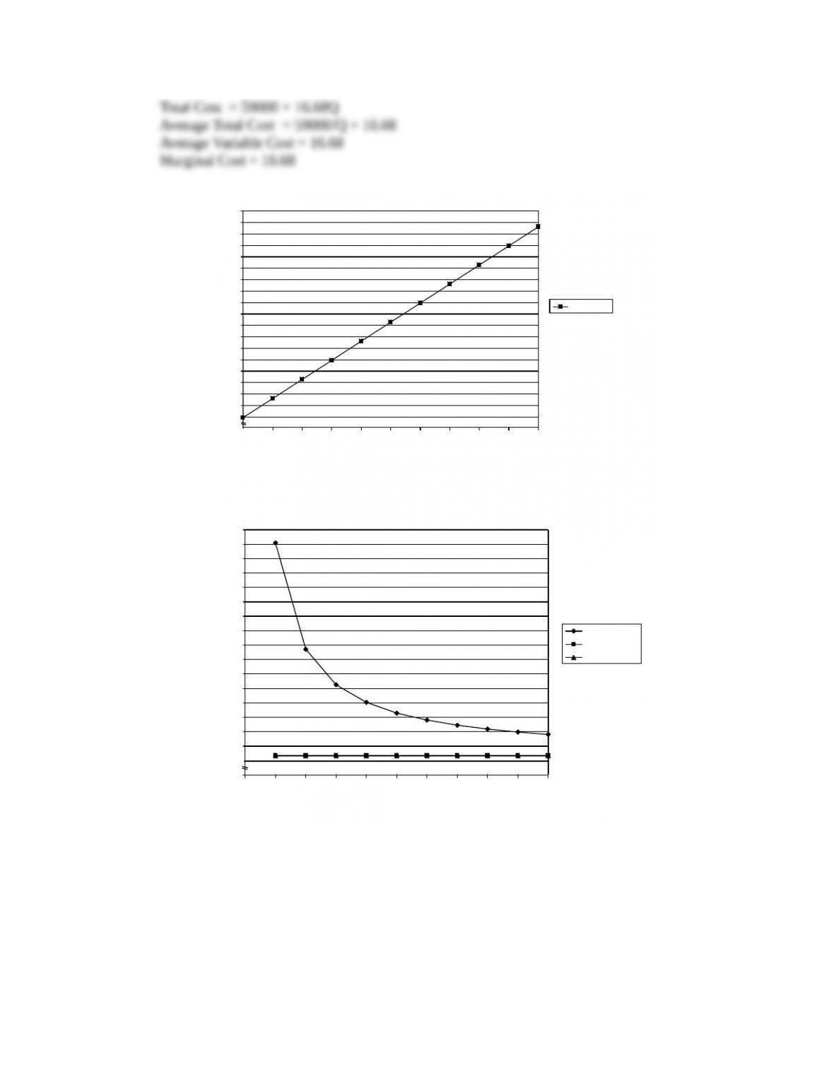
Figure 7.14
Figure 7.15
$ (thousands)
0
80
100
120
140
160
180
200
220
240
260
280
300
320
340
360
380
400
420
0 2000 4000 6000 8000 10000 12000 14000 16000 18000 20000
Q
Total Cost
60
$ (thousands)
0 2000 4000 6000 8000 10000 12000 14000 16000 18000 20000
Q
0
16
18
20
22
24
26
28
30
32
34
36
38
40
42
44
46
48
Av Total Cost
Av Var Cost
Marg Cost
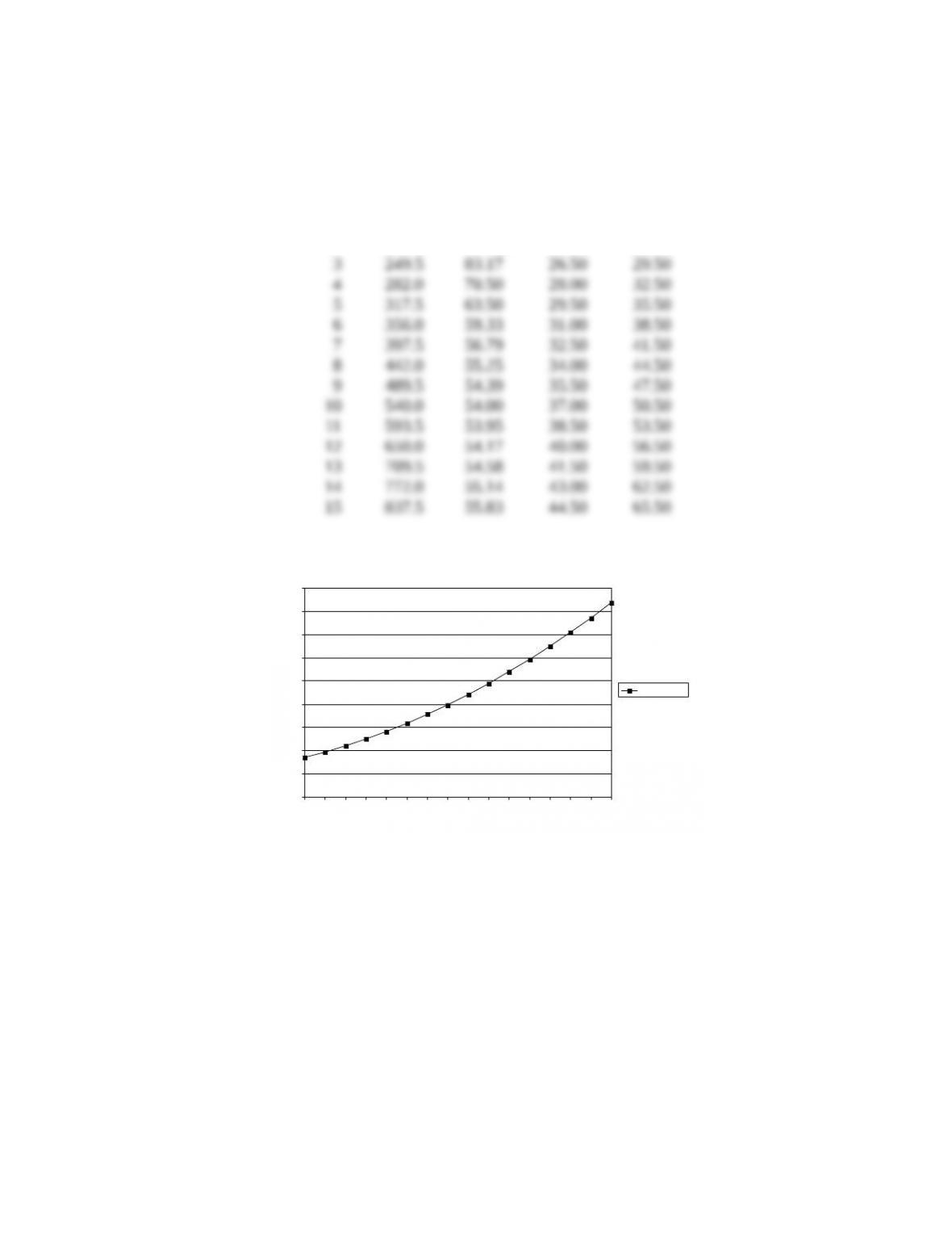
13. a.
Quantity Total
Cost
Average
Total
Cost
Average
Variable
Cost
Marginal Cost
0 170.0
1 193.5 193.50 23.50 23.50
2 220.0 110.00 25.00 26.50
b.
Figure 7.16
0
100
200
300
400
500
600
700
800
900
0 1 2 3 4 5 6 7 8 9 10 11 12 13 14 15
Q
Total Cost
$
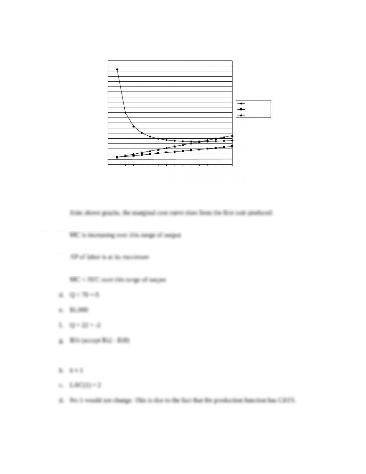
Figure 7.17
c. Big Horn’s cost curves do not include decreasing and constant marginal costs. As can be seen
14. a. Q > 40 (allow +-5 for this answer)
b. Q = 60 +-5
c. Q <= 60 +-5
15. a. CRTS
Q
$
20
30
40
50
60
70
80
90
100
110
120
130
140
150
160
170
180
190
200
210
0 1 2 3 4 5 6 7 8 9 10 11 12 13 14 15
Av Total Cost
Av Var Cost
Marg Cost
0
16.
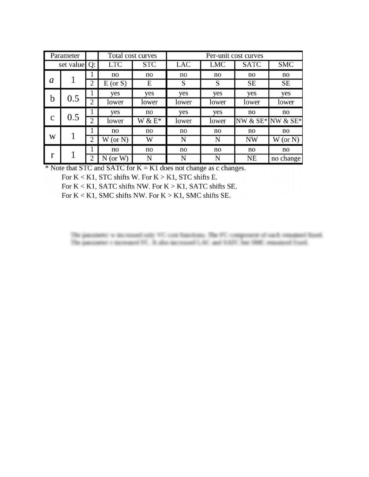
a. The CD exponents b and c altered RTS. They both created a situation of IRTS.
b. The parameter a decreased all cost functions.