Chapter 8 Competitive Firms and Markets 163
©2014 Pearson Education, Inc.
If the government imposes a $1.00 tax, the minimum average cost of production and hence the
equilibrium price increase by $1.00 (to $1.75), but the quantity produced by the firm does not. Market
quantity is
Q = 24 – p
Q = 22.25 units.
Each firm produces 0.5 units of output, and the total market quantity is 22.25. Therefore, there must
be 44.5 firms, from 22.25/0.5.
4.4 Assume each firm uses the same size plant in the short and the long run. Before the change in
4.5 To derive the expression for the elasticity of the residual or excess supply curve in Equation 8.17, we
differentiate the residual supply curve, Equation 8.16, Sr(p) = S(p) − Do(p), with respect to p to obtain
d dd
.
ddd
ro
S SD
ppp
= −
Let Qr = Sr(p), Q = S(p), and Qo = D(p). We multiply both sides of the differentiated expression by
p/Qr, and for convenience, we also multiply the second term by Q/Q = 1 and the last term by
Qo/Qo = 1:
dd d .
dd d
ro
o
r r ro
Q
S p S pQ D p
pQ pQQ pQQ
= −
164 Perloff • Microeconomics: Theory and Applications with Calculus, Third Edition
We can rewrite this expression as Equation 8.17 by noting that ηr = (dSt/dp)(p/Qr) is the residual
4.6 See the text for details:
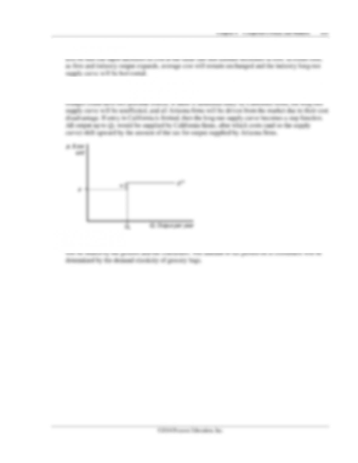
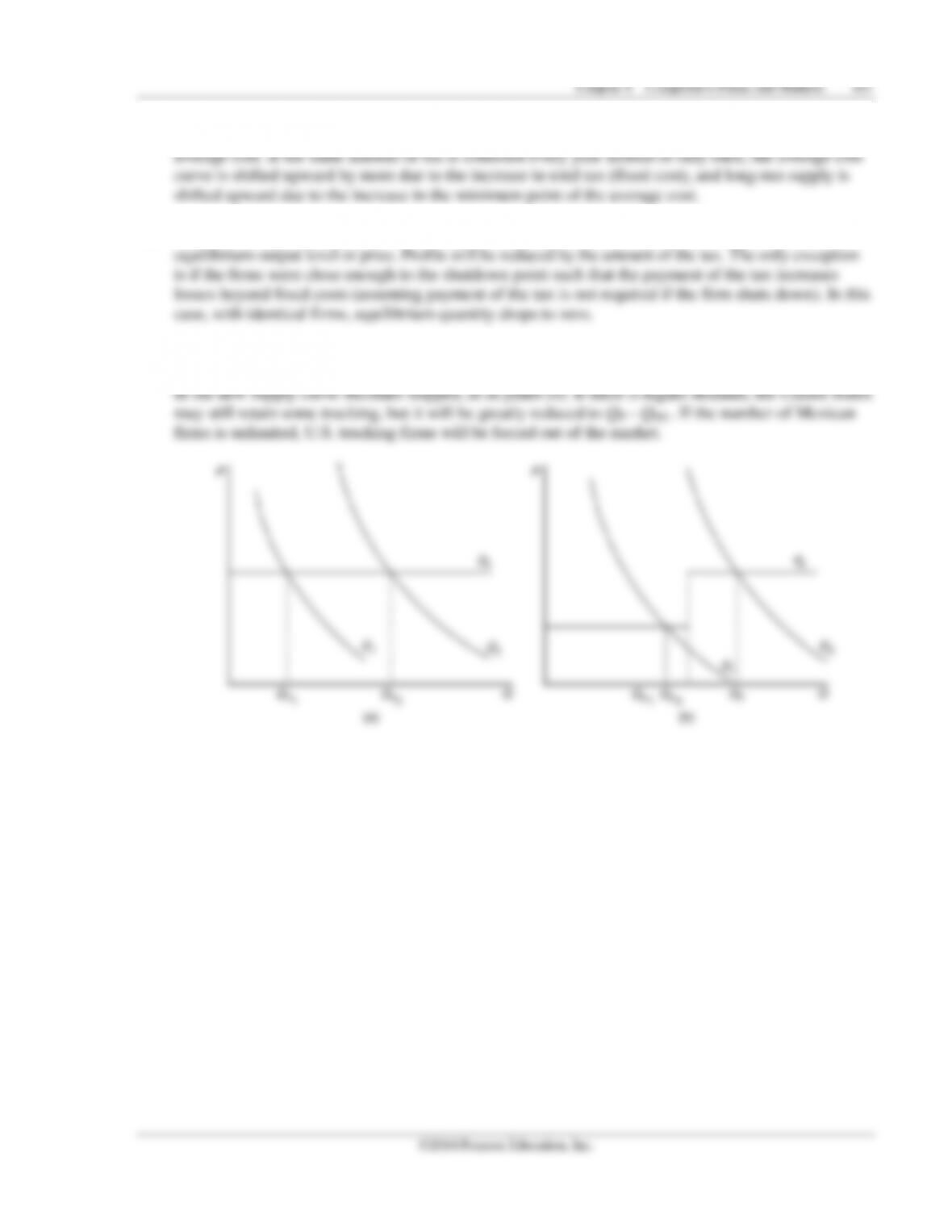
4.7 If importers were allowed to bring gas to California at a 15 cent surcharge, it would not alter the
normal equilibrium, as shown as p*, G*. However, in the event of a large leftward shift of the supply
166 Perloff • Microeconomics: Theory and Applications with Calculus, Third Edition
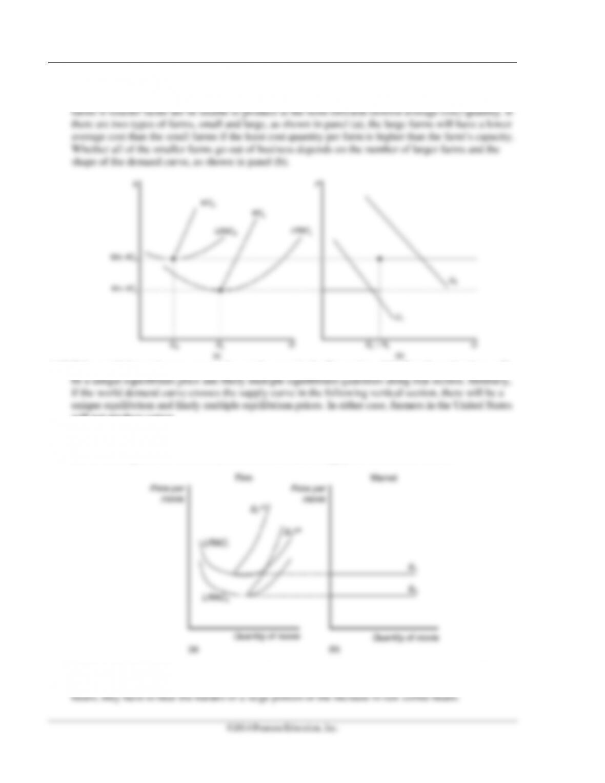
4.11 In the long run, farms will stay in business if their average cost is at or below the market price. With a
large annual fee (fixed cost), average costs per acre will be lower for the larger farms than for smaller
4.12 If the world demand curve crosses the supply curve in the flat section of the Brazil supply, there will
will not produce cotton.
4.13 Due to the lower average cost, the long run average cost curve shifts downward and firms’ supply
curves shift rightward. As a result, the horizontal market supply curve shifts downward.
4.14 One reason that firms increase the price of coffee only 14 percent may be that the demand of coffee is
elastic. On the other hand, since the roast coffee producers do not have good substitute for raw coffee
168 Perloff • Microeconomics: Theory and Applications with Calculus, Third Edition
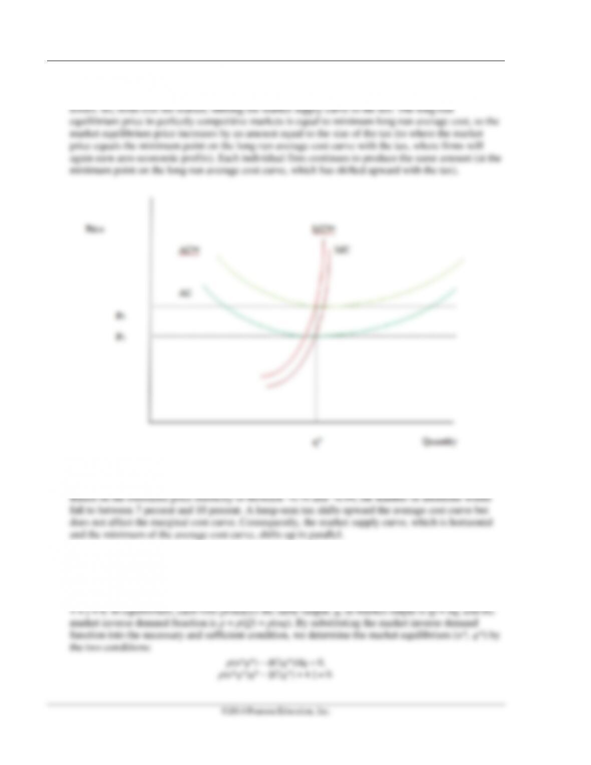
5.4 The per-unit tax shifts the marginal cost curve and the long-run average cost curve up by an amount
equal to the size of the tax (shown in the figure below). At the original market price, firms incur
5.5 Because the clinics are operating at minimum average cost, a lump–sum tax that causes the minimum
average cost to rise by 10 percent would cause the market price of abortions to rise by 10 percent.
5.6 Each competitive firm wants to choose its output q to maximize its after-tax profit: π = pq − C(q) −
+
.
Its necessary condition to maximize profit is that price equals marginal cost: p − dC(q)/dq = 0.
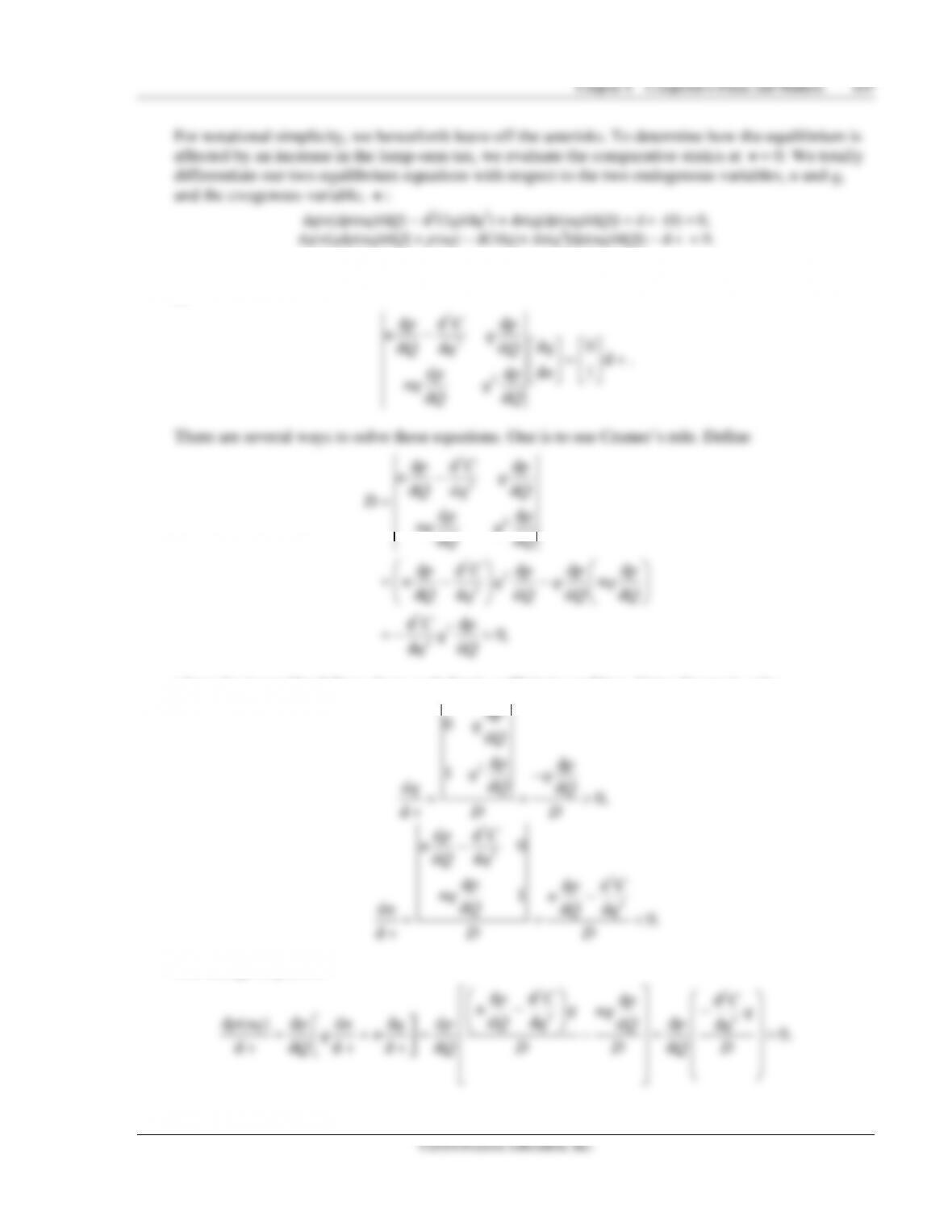
Industry supply is determined by entry, which occurs until profits are driven to zero (we ignore the
problem of fractional firms and treat the number of firms, n, as a continuous variable): pq − [C(q)
©2014 Pearson Education, Inc.
We can write these equations in matrix form (noting that p − dC/dq = 0 from the necessary condition)
as
2
2
2
dd d
d0
dd d d
d1
dd
dd
pC p
nq
q
Qq Q
n
pp
nq q
QQ
−
= +
.
There are several ways to solve these equations. One is to use Cramer’s rule. Define
2
2
2
22
2
22
2
dd d
dd d
dd
dd
dd d d d
dd d d d
dd
0,
dd
pC p
nq
Qq Q
Dpp
nq q
QQ
pC p p p
n q q nq
Qq Q Q Q
Cp
q
qQ
−
=
=−−
=−>
where the inequality follows from each firm’s sufficient condition. Using Cramer’s rule:
2
d
0d
dd
1d
dd0,
d
p
qQ
pp
qq
Q
qQ
DD
−
= = >
+
2
2
2
2
dd 0
dd
ddd
1
d
ddd 0.
d
pC
nQq
ppC
nq n
Q
nQq
DD
−
−
= = <
+
The change in price is
22
22
dd dd
dd
d( ) d d d d d
dd
0.
d dd d d d
pC pC
nq
nq q
Qq
p nq p n q p p
Qq
qn
Q Q D D QD
−−
= += − = >
+ ++