Chapter 8 Competitive Firms and Markets 153
8. True or false, explain your answer. “If all firms in an industry have identical variable cost, but each
pays a different one–time fee to enter the market, all firms will produce identical quantities of output.”
9. If each competitive firm in an industry has the short–run cost function C = 50 + 5q + q2, and the market
price is $35, what is the profit–maximizing output level for each firm? What is the total revenue?
What are the profits?
10. Suppose, in Question 9, that fixed costs were $250 instead of $50. How does this change affect the
firm’s output decision and profits? Should the firm continue to operate?
11. How does a firm decide whether to shut down production if it has zero fixed cost? What is the
implication on entry and exit in this industry?
12. Using equation 8.5 for the elasticity of excess supply, discuss the relationship between market supply
elasticity and excess supply? Which one is higher? Under what circumstance will these two be the same?
Answers to Additional Questions and Problems
1. Advertising is pro–competitive when it provides information to consumers about prices and product
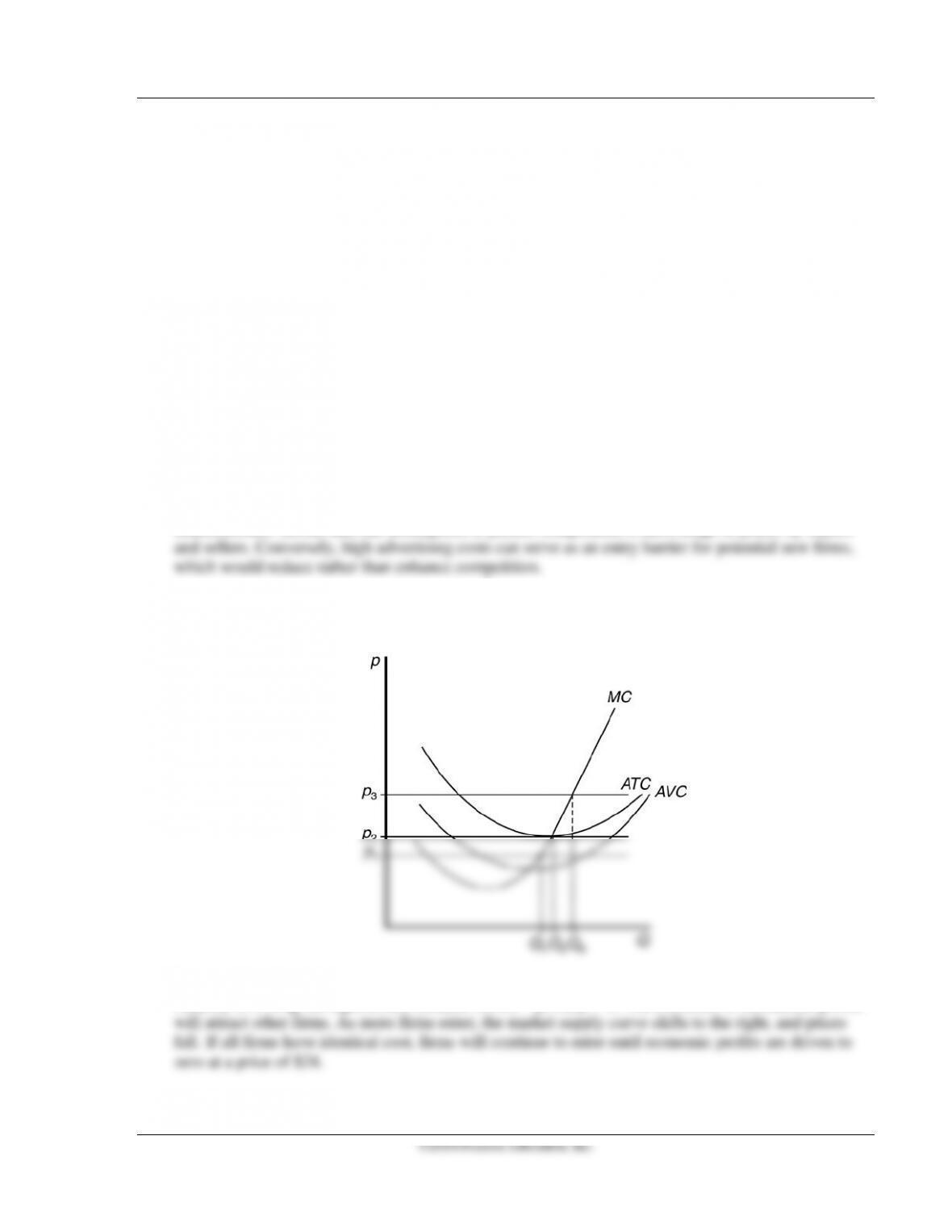
2. At p3, the firm makes positive profits. At p2, the firm breaks even, and at p1, the firm realizes losses
that are less than fixed costs.
3. Such a firm would be producing 110 units per year at a price of $35. In this case, the firm but not the
154 Perloff • Microeconomics: Theory and Applications with Calculus, Third Edition
4. Unless you are the only farmer who has access to this new technology, this is not good news. Because
the fertilizer producers want to maximize their own profits, they will try to sell the new product to all
farmers. Thus each farm will be able to increase production per acre. No individual farm would want
5. The marginal cost equation is MC = 2q. When p = $30, q* = 15, p = $100. When p = $20, q* = 15,
6. The residual demand elasticity is calculated using Equation 8.2.
( )
1
io
nn
εε η
= −−
= −37.5 − 24 = −61.5.
7. This statement is false. Diminishing marginal returns, which lead to increasing marginal cost, are a
8. This statement is true. Fixed costs are irrelevant when determining output levels in the short run. All
9. Set MC = MR and solve.
MC = 2q + 5
10. As in Question 9, set MC = MR and solve. Output is unchanged, but profits fall.
MC = 2q + 5
11. With zero fixed cost, the firm will shut down production when the price is below the minimum
Chapter 8 Competitive Firms and Markets 155
©2014 Pearson Education, Inc.
12. Since θ is between zero and one, and
ε
is usually negative, we have
ητ
=
η
/
θ
−
ε
(1 −
θ
)/
θ
>
η
. For
ε
< 0, we have
η
=
ητ
if and only if
θ
= 1. In other words, only when this country is the only one
producing this good.
Answers to Exercises in the Text
1.1 A market is considered to be perfectly competitive if consumers believe that all firms in the market
sell identical products, if firms freely enter and exit the market, if buyers and sellers know the prices
charged by firms, and if transaction costs are low. The characteristics of this restaurant market that
1.2 If buyers know the prices that other firms charges—the market price—a firm cannot raise its price
without losing its customers. In contrast, if consumers do not know the prices that other firms charge,
2.1 The shutdown rule states that a firm should shut down when it can avoid additional losses by doing
2.2 a. Fixed cost is sunk in the short run. Therefore, if the firm shuts down it loses the fixed cost, which
is F = $600. However, if it continues to produce, it only loses $100. So, it should not shut down.
2.3 How much the firm produces and whether it shuts down in the short run depends only on the firm’s
variable costs. (The firm picks its output level so that its marginal cost—which depends only on
variable costs—equals the market price, and it shuts down only if market price is less than its
156 Perloff • Microeconomics: Theory and Applications with Calculus, Third Edition
©2014 Pearson Education, Inc.
opportunity costs—the amount for which the firm could rent the plant to someone else—and not on
historical payments.
2.4 The logic behind the first claim is that the firm chooses not to charge the full price of one of the
inputs, the rent. The logic for the second claim is that since it is charged a lower price for one of the
inputs, the output price is also lower.
2.5 The first-order condition to maximize profit is the derivative of the profit function with respect to q
3.1 Revenue is a straight line because the firm is a price taker. The slope of the revenue curve is equal to
the price. The slope of the profit curve when profit is maximized is zero (because it’s at a maximum
3.2 The firm’s profit is
π = pq – (10 + 10q + q2).
3.3 Marginal cost is computed by taking the derivative dC/dq. Profits are maximized by setting
3.4 The firm’s after–tax profit is
π = pq – (10 + 10q + q2) – τq.
Chapter 8 Competitive Firms and Markets 157
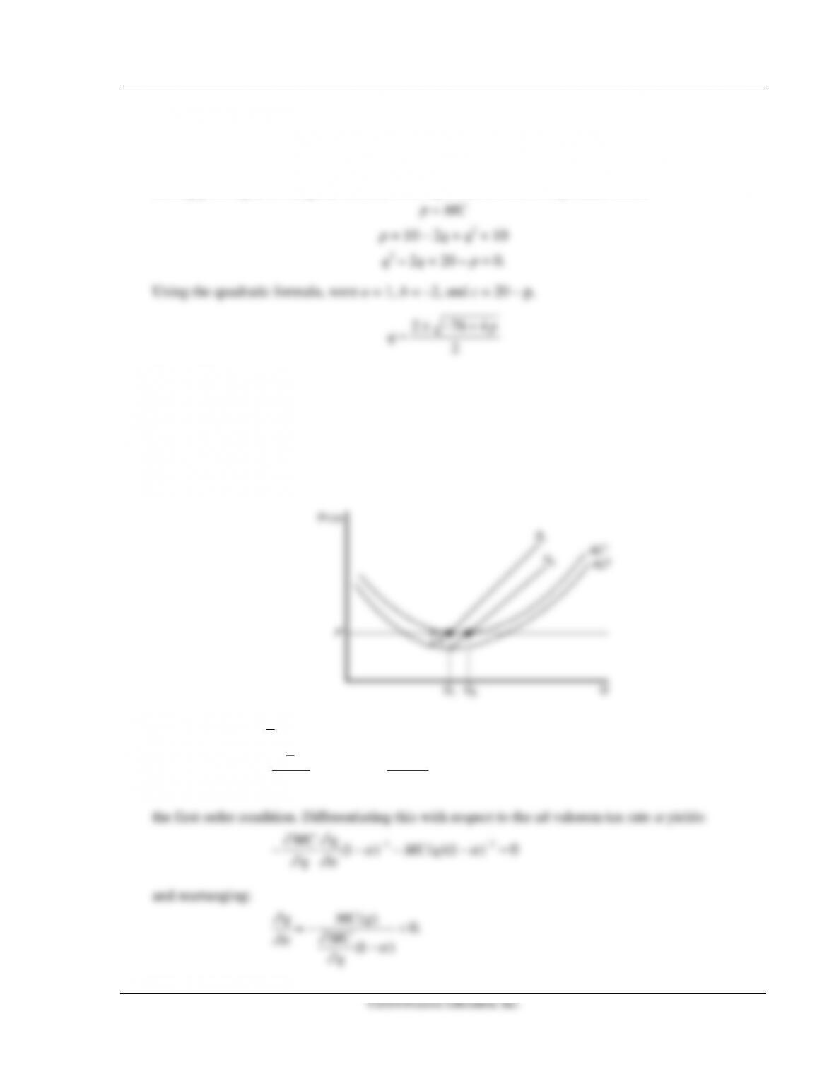
3.5 The after-tax cost function is C = 100 + 10q – q2 + (1/3)q3 + 10q. The firm will maximize profit by
producing the quantity where price equals marginal cost. Marginal cost (MC) is
MC = 10 – 2q + q2 + 10.
Setting price equal to marginal cost, the firm’s production rule is to produce where
2
for p > 19.
3.6 In the long run, the average cost curve will shift down by the amount of a per unit subsidy, and the
firm’s marginal cost curve, or supply curve, will shift right. Since the market price will not change
significantly with lower costs for one firm, the firm will increase its output to where its new marginal
cost equals market price, and its profits will go from the market equilibrium of zero to a positive
amount.
3.7 After-tax profit is
(1 ) ( )pq C q
πα
=−−
and the profit-maximizing output after the tax is imposed is:
() ()
(1 ) 0
q Cq
p
qq
∂π ∂
α
∂∂
=−− =
or
1
( )(1 ) 0,p MC q
α
−
− −=
(1 )
MC
q
∂
∂α α
∂
−
158 Perloff • Microeconomics: Theory and Applications with Calculus, Third Edition
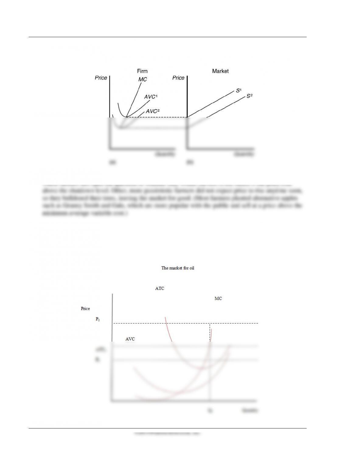
3.8 The lower of average minimum variable cost will extend the firm’s supply curve downward. As a
result, the market supply curve shifts rightward.
3.9 Some farmers did not pick apples so as to avoid incurring the variable cost of harvesting apples.
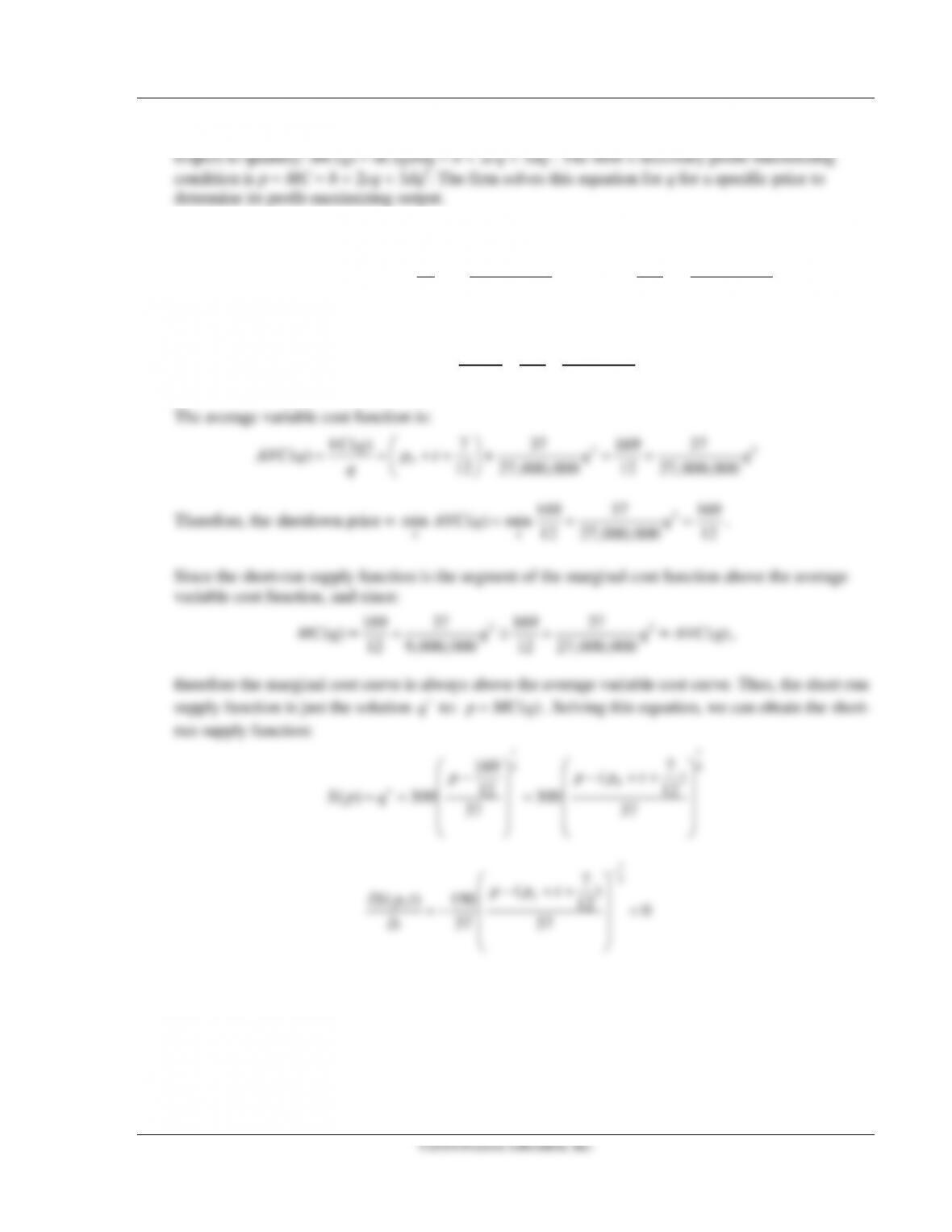
3.10 It may be that at a relatively low price of oil, such as p1, oil extraction is not profitable (because the
price is lower than the average total cost of producing the profit–maximizing quantity). When
gasoline prices spike, the price of oil rises. Assume the price of oil rises to p2. At this price, the profit–
maximizing quantity (where price equals marginal cost) is Q2. Production is now profitable because
the price (p2) is greater than the average total cost of producing Q2 units.
Chapter 8 Competitive Firms and Markets 159
3.11 The competitive firm’s marginal cost function is found by differentiating its cost function with
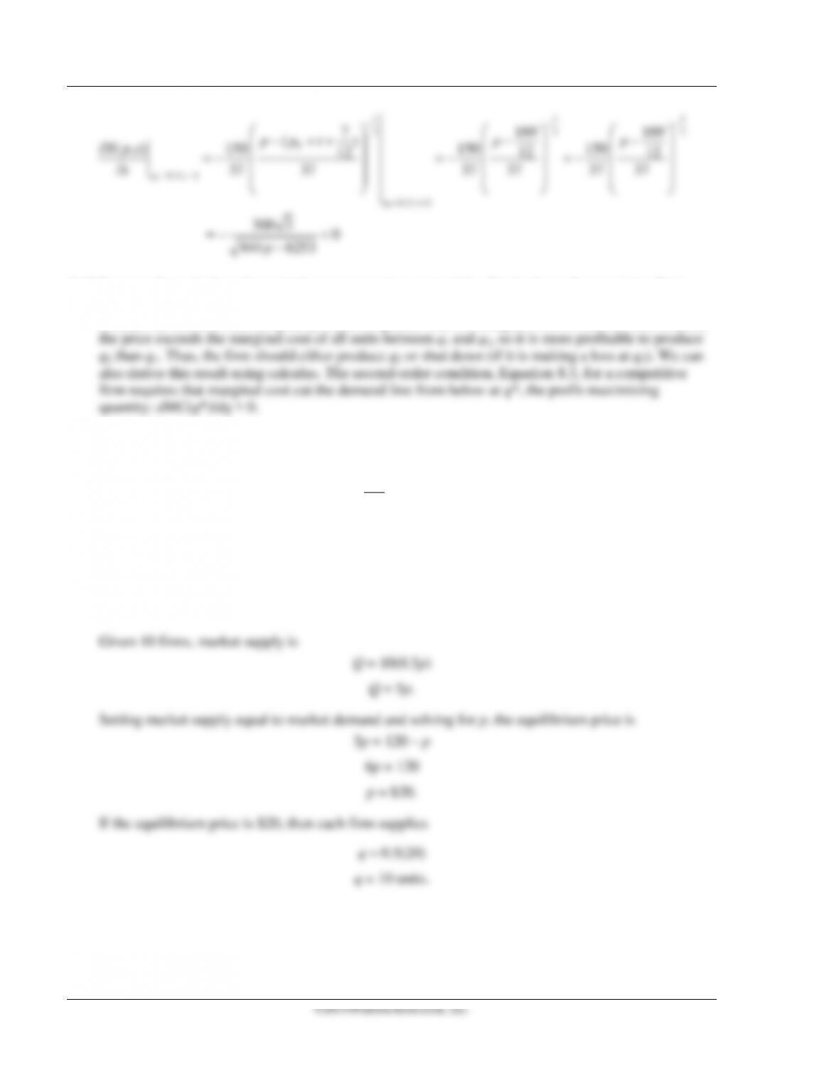
3.12 The total cost function is:
33
7 37 169 37
( ) 6860 6860
12 27,000,000 12 27,000,000
T
Cqptqqqq
= + ++ + = + +
,
then the marginal cost function is:
2
( ) 169 37
() 12 9,000,000
Cq
MC q q
q
∂
= = +
∂
37 37
t
∂
160 Perloff • Microeconomics: Theory and Applications with Calculus, Third Edition
©2014 Pearson Education, Inc.
1 11
2 22
11.5, 2
11.5, 2
7 169 169
()
( , ) 150 150 150
12 12 12
37 37 37 37 37 37
300 3 0
444 6253
T
T
T
pt
pt
ppt p p
S pt
t
p
− −−
= =
= =
− ++ − −
∂=− =−=−
∂
=−<
−
3.13 Suppose that a U-shaped marginal cost curve cuts a competitive firm’s demand curve (price line)
from above at q1 and from below at q2. By increasing output to q1 + 1, the firm earns extra profit
because the last unit sells for price p, which is greater than the marginal cost of that last unit. Indeed,
3.14 Each firm maximizes profit by producing where price equals marginal cost. The marginal cost of
production is
2
Cq
q
∂=
∂
.
Setting price equal to marginal cost (MC) and solving for q,
p = MC
p = 2q
q = 0.5p.
Chapter 8 Competitive Firms and Markets 161
©2014 Pearson Education, Inc.
Substitute the market equilibrium price into the market demand curve and solve for Q to find the
market quantity:
Q = 120 – p
Q = 120 – 20
Q = 100 units.
3.15 Each firm maximizes profit by producing where price equals marginal cost. The marginal cost of
production is
2
Cq
q
∂=
∂
+ 2.40.
Setting price equal to marginal cost (MC) and solving for q,
p = MC
p = 2q + 2.40
q = 0.5p – 1.2.
162 Perloff • Microeconomics: Theory and Applications with Calculus, Third Edition
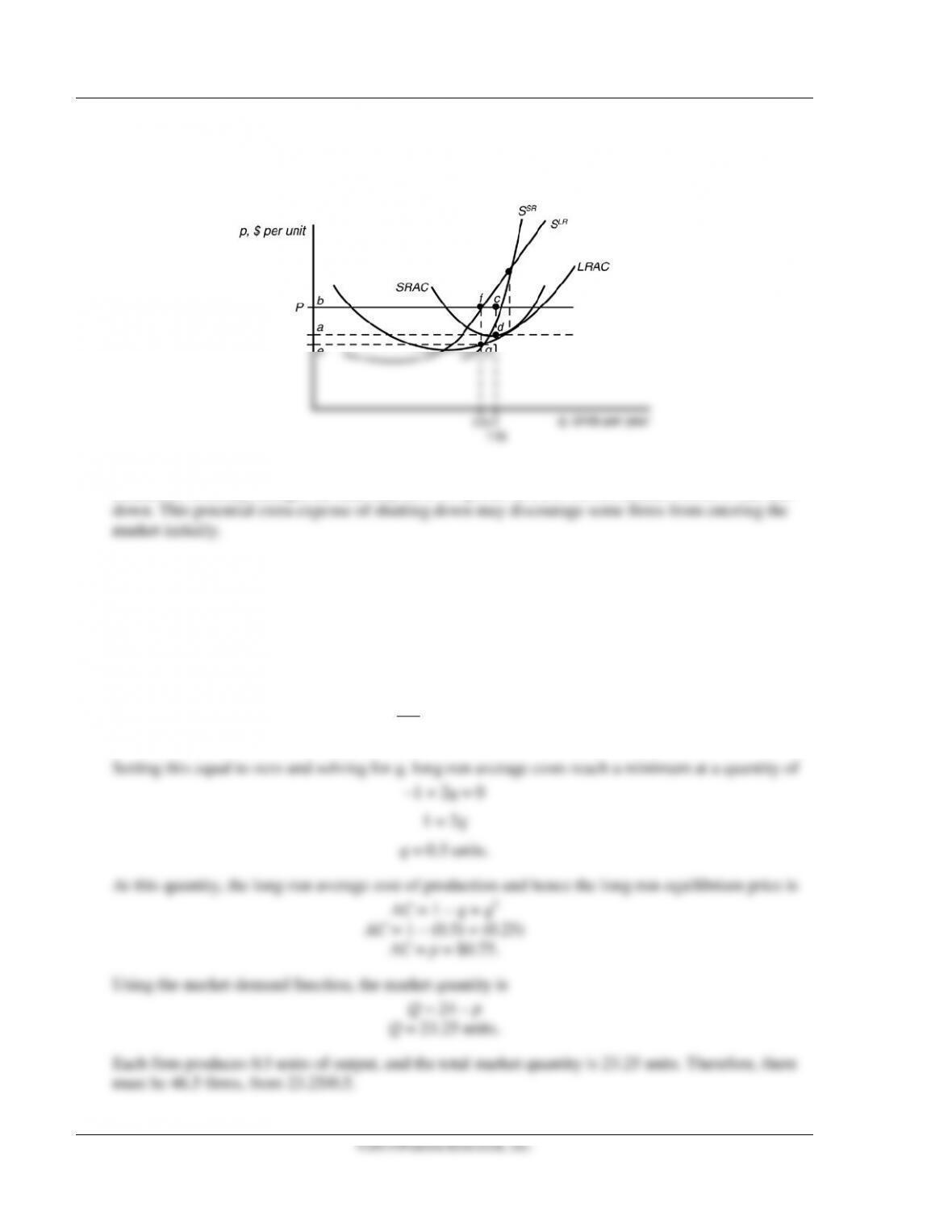
4.1 In this case the firm is producing more than the long-run profit-maximizing output level of 110.
Profits are currently equal to area abcd, but would be increased to area ebfg with the optimal plant
size.
4.2 The shutdown notice reduces the firm’s flexibility, which matters in an uncertain market. If
conditions suddenly change, the firm may have to operate at a loss for six months before it can shut
4.3 Assume the cost function is C = q – q2 + q3. The long–run equilibrium price will be where the long–
run average cost curve is at a minimum. Average costs (AC) are
AC = –1q + q2.
To find where average costs reach a minimum, take the derivative of the average cost function with
respect to q:
C
q
∂
∂
= –1 + 2q.