
148
©2014 Pearson Education, Inc.
Chapter 8
Competitive Firms and Markets
Chapter Outline
8.1 Perfect Competition
Price Taking
Why a Firm’s Demand Curve Is Horizontal
Large Number of Small Firms and Consumers
Identical Products
Full Information
Negligible Transaction Costs
Free Entry and Exit
Perfect Competition in the Chicago Commodity Exchange
Deviations from Perfect Competition
Derivation of a Competitive Firm’s Demand Curve
Why Perfect Competition Is Important
8.2 Profit Maximization
Profit
Two Steps to Maximizing Profit
Output Rules
Shutdown Rules
8.3 Competition in the Short Run
Short-Run Competitive Profit Maximization
Short-Run Output Decision
Solved Problem 8.1
Short-Run Shutdown Decision
Application: Oil, Oil Sands, and Oil Shale Shutdowns
Short-Run Firm Supply Curve
Tracing Out the Short-Run Supply Curve
Solved Problem 8.2
Factor Prices and the Short–Run Firm Supply Curve
Short-Run Market Supply Curve
Short-Run Market Supply with Identical Firms
Short-Run Market Supply with Firms That Differ

Chapter 8 Competitive Firms and Markets 149
©2014 Pearson Education, Inc.
Short-Run Competitive Equilibrium
Solved Problem 8.3
8.4 Competition in the Long Run
Long-Run Competitive Profit Maximization
Long-Run Firm Supply Curve
Application: The Size of Ethanol Processing Plants
Long-Run Market Supply Curve
Entry and Exit
Application: Fast-Food Firms Entry in Russia
Long-Run Market Supply with Identical Firms and Free Entry
Long-Run Market Supply When Entry is Limited
Long-Run Supply When Firms Differ
Application: Upward-Sloping Long-Run Supply Curve for Cotton
Long-Run Market Supply When Input Price Vary with Output
Long-Run Market Supply Curve with Trade
Application: Reformulated Gasoline Supply Curves
Solved Problem 8.4
Long-Run Competitive Equilibrium
Teaching Tips
Chapter 8 begins the study of markets. You might begin this section by talking with the class about market
structure in its broadest terms. Introduce the spectrum of market structures by briefly defining the competitive,
monopolistically competitive, oligopoly, and monopoly market structures. By doing so, you will answer some
questions in advance about markets that do not fit into the competitive model.
If you ask the students for a list of characteristics that describe a competitive market, or a firm in such a
market, you are likely to get a combination of assumptions (e.g., free entry and exit, perfect information)
and outcomes (e.g., lack of market power, zero long-run profits). Probably the most common mistake that
students make at this stage is to confuse assumptions and outcomes. It is important that students understand
that price –taking behavior is not assumed, or a choice that firms make, but an outcome that is driven by
the assumptions that are made.
Before beginning the material on short– and long-run profit maximization, you may want to review the
difference between economic profit and business profit. Throughout the chapter, the text uses the word
profit to mean economic profit.
Most of the material on short-run profit maximization is straightforward and should not be cause for much
confusion. The possible exception is the shutdown rule. You may find that no matter how much you
emphasize to the class that the firm must cover its variable cost, some still remember it as the firm needing
to cover fixed cost to avoid shut down. You may reduce this confusion by the use of a simple example.
You might describe a firm where the only fixed cost is a mortgage payment and the only variable cost is
the payroll. It makes intuitive sense that as long as the firm can make the payroll every week, even if it can
only pay part of its mortgage, it can hang on and hope for higher prices. However, once the firm can’t even
cover its payroll, it must shut down.

150 Perloff • Microeconomics: Theory and Applications with Calculus, Third Edition
©2014 Pearson Education, Inc.
When covering the firm and market short-run supply curves, you might emphasize that the point at which
the supply curve is cut off at the lower end is not arbitrary but a function of the average variable cost curve
and shutdown point. The section of the chapter that covers short-run supply contains a good discussion of
the effect of changes in input prices and taxes on equilibrium output levels. You may want to work through
some examples, such as the supply of vegetable oil example in Figure 8.6.
When discussing the long run, it is vital that the class understands that the assumptions of the model,
particularly free entry and exit, are the force that drives the competitive engine. Firms are forced by the
continual push of actual or potential competition to produce efficiently and maximize profits. You can use
statistics from agriculture to show that farmers have been forced over time to become increasingly efficient
producers in order to remain solvent. As technology increases, output per acre increases, increasing output
and reducing prices. Falling prices create the incentive to cut costs. Cutting costs increases supply, which
creates even more downward pressure on prices. The cycle is continuous, as farmers face constant downward
pressure on long-run profits. This has caused a continuous increase in average farm size, the disappearance
of many small, unproductive farms, and enormous increases in productivity. For example, from 1955 to
1986, labor input per acre of corn fell by over three times, while output per acre more than doubled. During
the same time period, labor input per hundredweight of turkeys fell from 4.4 to 0.2.1 This is a good place
to remind the class of the normative economic issues created by the force of markets. Although the efficiency
of the agriculture industry results in low food prices, they can be forced so low that many family farms cannot
survive. You might try to get the class to weigh in on whether normative solutions such as price supports,
which save farms but create higher prices, are a good thing or should be abolished. You may also want to
discuss the computer industry, where prices for PC computing power have fallen at an average rate of
about 30 percent per year. In this case, despite the fact that some of the assumptions of the perfectly
competitive market are not met, consumers still derive great benefit from the forces of markets.
Canada’s Response to Increased International Competition
in World Agriculture Markets2
Canada is a major producer of wheat. Because the agricultural sector is so large relative to the size of the
population, they are also major exporters. Not surprisingly, they push hard for open access to foreign markets.
Between 1990 and 2000, agricultural goods and food byproduct exports increased by more than 100
percent. To continue this trend, they will have to not only win the battle for lower tariffs but also battle
falling world prices brought about by increases in production (farmed acreage) and productivity.
As noted above, productivity in agriculture has skyrocketed due to increases in mechanization, fertilizers,
and biotechnology. In some areas, soil that was previously thought untellable is now planted acreage.
In addition, the recent economic downturn and former Soviet state’s inability to pay for imports have
dampened world demand. The effect on wheat prices has been dramatic. Prices have fallen roughly 75
percent since 1970. Although agricultural subsidies in the United States and the European Union are
commonly blamed as major culprits in the fall of grain prices, they may only be responsible for one-fourth
of the decline. As low-cost producers continue to emerge throughout the world, Canada’s agricultural
sector will continue to experience the heavy pressure of falling prices. In order to remain competitive,
Canadian farmers will have to continue to increase their own productivity. Thus the problem of U.S.
farmers and their continual contribution to lower prices in an effort to maintain profitability through
productivity increases is played out on the world stage as well.
1U.S. Department of Agriculture statistics, reported in Agriculture by Daniel B. Suits in The Structure of American Industry, ninth
edition, Adams and Brock, eds. Prentice Hall, Englewood Cliffs, NJ. 1995:21.
2 Competition and Subsidies in Global Markets, at http://www.agr.gc.ca/cb.apf/bgd_comp_e.html.

Chapter 8 Competitive Firms and Markets 151
©2014 Pearson Education, Inc.
1. Should international financial institutions such as the WTO intervene in international agriculture
markets to stabilize prices? Who would be helped, and who would suffer if it did?
2. Could the Canadian government act alone to affect the fate of Canadian farmers on international
markets? If so, how?
Additional Applications
Barriers to Exit—The Steel Trap3
If firms incur a cost to exit the market, they may not shut down in the short run even if their revenues do
not cover variables costs. The firms stay in operation, at least for a while, so that they can avoid paying the
exit costs.
For decades, many integrated U.S. steel mills—factories that produce steel from iron ore—were operating
at losses. Before the 1950s, U.S. firms could produce at lower costs than international rivals despite having
high wages because their mills were more productive and abundant supplies of coal and iron ore kept their
energy and material costs relatively low. In the 1950s and 1960s, discoveries of rich iron ore sources, lower
wages, and newly built, state–of–the–art mills enabled many foreign steel firms to produce at lower cost than
U.S. firms. As a result, the share of worldwide sales of U.S. integrated steel firms fell from 90 percent in
1960 to less than 65 percent in the 1980s.
U.S. firms have been too slow to leave the market. Not until the late 1970s did Youngstown Sheet & Tube
and the United States Steel Corporation in Youngstown, Ohio close. The next closing did not occur until
1982. Rather than close, firms have continued to operate aging, inefficient, and unprofitable plants.
A steel firm faces substantial costs in closing a mill and terminating contracts. Union contracts obligate the
firm to pay workers severance pay, supplemental unemployment benefits, and make payments to cover
additional pensions and insurance benefits in the future. Usually, union members are eligible for pensions
when their age plus years of service equals 75; however, workers laid off due to plant closings are eligible
when their age plus years of service equals 70. Thus by not closing plants, firms can substantially reduce
pension payments. The United States Steel Corporation’s cost of closing down various operations in 1979
was $650 million, of which about $415 million—or $37,000 per laid-off worker—was labor related. These
costs have risen 45 percent since then.
Because they avoided shutting down to avoid exit costs, U.S. steel mills have sold most products at prices
below average variable cost since the 1970s. For example, in 1986, the average variable cost of hot-rolled
sheets per ton was $305 and the average cost was $406, but the price was only $273. Many of these mills
stayed in business for decades despite sizable losses. Eventually, these mills will close unless the recent
increase in profitability in the industry continues.
1. Can you think of other firms or industries that would suffer large shut-down costs? What would be
the source of these costs?
2. Is it possible that the firms are playing a “waiting game” to see if others will drop out before them?
Under what circumstances might this allow a remaining firm to become profitable again?
3From Mary E. Deily, Exit Barriers in the Steel Market, Economic Review, 24(1), Quarter 1, 1988:10–18.

152 Perloff • Microeconomics: Theory and Applications with Calculus, Third Edition
©2014 Pearson Education, Inc.
Discussion Questions
1. Give some examples of markets that, based on their characteristics, are likely to be competitive.
2. Should firms use accounting profits or economics profits when deciding how much to produce?
3. Are entry barriers ever desirable? Why?
4. Give examples of avoidable costs and sunk costs.
5. Is competition desirable? Why? (This topic is discussed in the next two chapters.)
6. Give examples of exit barriers. How do they limit or impede exit?
7. A lump–sum tax does not affect a firm’s marginal cost. Does it alter the short-run competitive
market equilibrium?
8. How do fixed costs affect firms’ behaviors in the short run?
9. Should a competitive firm care about the behavior of any one of its rivals (as opposed to all of them
collectively)?
Additional Questions and Problems
1. Under what circumstances would advertising be pro-competitive? Anti–competitive?
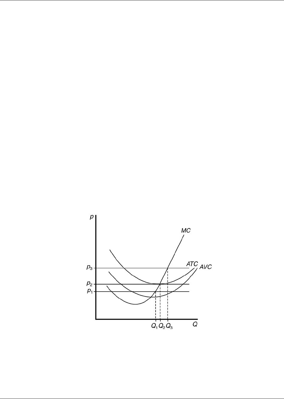
2. Draw a graph showing the average total, average variable, and marginal cost curves for a typical firm.
Draw in three prices that result in the firm making positive profits, breaking even, and making negative
profits that are less than fixed costs.
3. Suppose your firm is in a competitive industry in long–run equilibrium making substantial long-run
profits (as in Figure 8.11). State specifically what will occur as the industry moves toward long-run
equilibrium.
4. Suppose you are a wheat farmer, and the local fertilizer salesperson informs you that a new product is
available that could boost your output by 15 percent. Is this good news or bad news? Why?
5. Suppose a perfectly competitive firm has the short–run cost function C = 125 + q2. Use the derivative
formula or marginal cost to determine the firm’s output level and profit at prices of $30 and $20. At
what price does the firm reach the shutdown point?
6. Suppose there are 25 firms in the sandals market, in which market demand elasticity is –1.5. The
elasticity of supply is 1. A single firm in this industry decides that because there are only 24 competitors,
it might be a good idea to increase prices by 1 percent. Use the information in Appendix 8A to show
the outcome of this decision.
7. True or false, explain your answer. “The lawn chair industry is a constant cost industry. This means
that the law of diminishing returns does not operate, and the marginal cost curve is flat.”
Chapter 8 Competitive Firms and Markets 153
©2014 Pearson Education, Inc.
8. True or false, explain your answer. “If all firms in an industry have identical variable cost, but each
pays a different one–time fee to enter the market, all firms will produce identical quantities of output.”
9. If each competitive firm in an industry has the short–run cost function C = 50 + 5q + q2, and the market
price is $35, what is the profit–maximizing output level for each firm? What is the total revenue?
What are the profits?
10. Suppose, in Question 9, that fixed costs were $250 instead of $50. How does this change affect the
firm’s output decision and profits? Should the firm continue to operate?
11. How does a firm decide whether to shut down production if it has zero fixed cost? What is the
implication on entry and exit in this industry?
12. Using equation 8.5 for the elasticity of excess supply, discuss the relationship between market supply
elasticity and excess supply? Which one is higher? Under what circumstance will these two be the same?
Answers to Additional Questions and Problems
1. Advertising is pro–competitive when it provides information to consumers about prices and product
characteristics. Recall that one assumption of perfect competition is knowledge of prices by buyers
and sellers. Conversely, high advertising costs can serve as an entry barrier for potential new firms,
which would reduce rather than enhance competition.
2. At p3, the firm makes positive profits. At p2, the firm breaks even, and at p1, the firm realizes losses
that are less than fixed costs.
3. Such a firm would be producing 110 units per year at a price of $35. In this case, the firm but not the
industry is in long-run equilibrium because LRMC = p, but p > 0. The existence of substantial profits
will attract other firms. As more firms enter, the market supply curve shifts to the right, and prices
fall. If all firms have identical cost, firms will continue to enter until economic profits are driven to
zero at a price of $24.