132 Perloff • Microeconomics: Theory and Applications with Calculus, Third Edition
9. If input prices are w = 3, and r
=
2, and q = 10KL, what is the least cost input combination required
to produce 60 units of output? How would input usage change if output is increased to 240 units?
Sketch the solutions on a graph.
10. In Question 8, suppose the government, in an effort to increase employment, offers firms in this
industry a $1 per unit subsidy. How would this affect input usage (assume q = 60). How is this likely
to affect employment in the capital goods (K) industry?
11. Two firms currently produce the goods q1 and q2 separately. Their cost functions are C(q1) = 25 + q1,
and C(q2) = 35 + 2q2. By merging, they can produce the two goods jointly with costs described by the
function C(q1, q2) = 45 + q1 + q2. Are there scope economies in this case that would justify the merger?
12. Suppose the production function is Q = a min(K, L), where a is a positive constant, the price of
capital good is $10 per unit, and labor cost is $10 per worker hour. What is the optimal combination
of capital and labor?
13. In Question 12, suppose the production function is Q =
ac min(K, L), where a is a positive constant
and c > 1. The price is of capital good is $10 per unit, and labor cost is $10 per worker hour. What is
the optimal combination of capital and labor? Does the production function have an increasing,
constant, or diminishing return to scale?
Answers to Additional Questions and Problems
1. Table 7.2
q VC L AVC MC
1
20
1
20
20
2
40
2
20
20
3
60
3
20
20
4
80
4
20
20
5
120
6
24
40
6
160
8
26.67
40
7
240
12
34.29
80
Chapter 7 Costs 133
2. The statement is false because the individual has failed to account for the opportunity cost of his or
3. By expensing all costs of capital improvements in the current period, the firm will be biased toward
increases in labor rather than capital. Capital improvements will only be made when their cost is less
4. To find this point, recall that the marginal cost curve crosses the average cost curve at the minimum
point of the average cost curve. To find the minimum, take the derivative of AC, and set it equal to zero.
5. MC and MPL are inverted images of one another. For a typical production function, with fixed input
prices, marginal product rises at first, then falls as diminishing returns set in. The marginal cost curve
6. The equation for marginal cost is Q2 − 6Q + 15. To find the minimum, you could either take the
7. The output level Q* represents capacity.
8. As shown in Equation 7.9, minimizing cost requires that MRTS = w/r. Since MRTS = MPL/MPK,
set the ratio of marginal products equal to the ratio of input prices, then substitute into the output
constraint.
134 Perloff • Microeconomics: Theory and Applications with Calculus, Third Edition
©2014 Pearson Education, Inc.
K* = 20
C = 4(5) + 1(20) = 40
If capital is fixed at 16 units, least cost production is not possible. Instead, labor must be increased to
6.25 units. Total cost increases from $40 to $41.
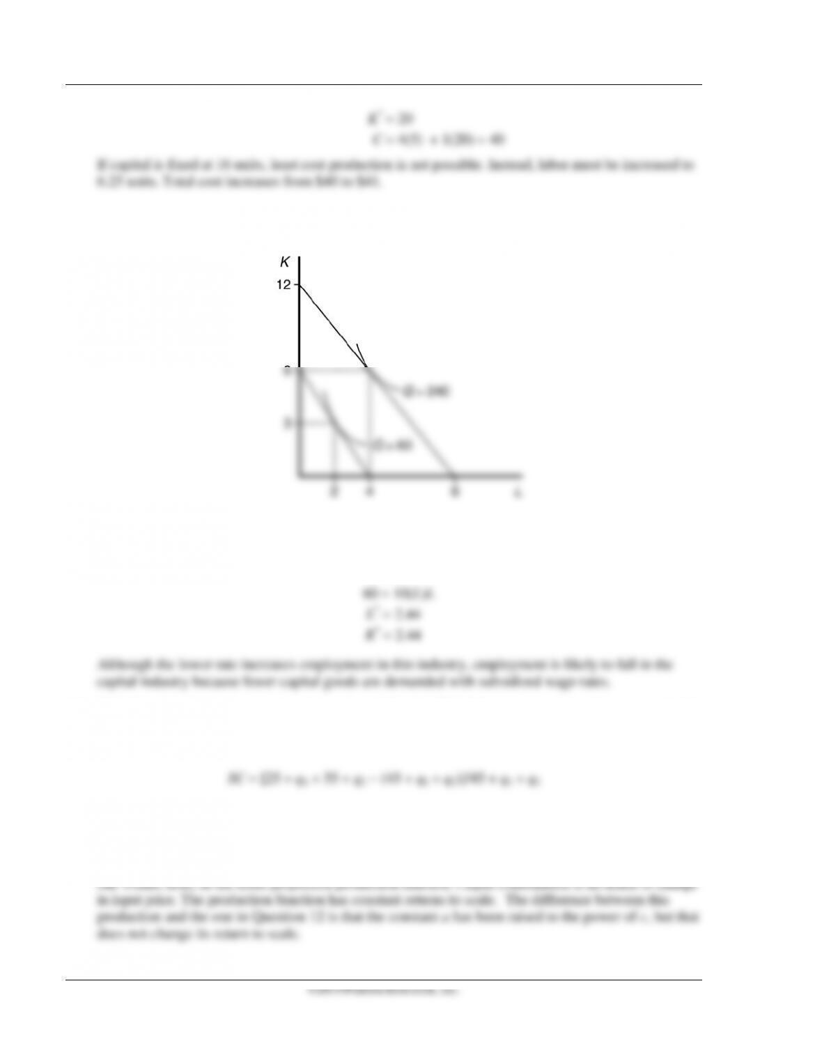
9. Solve as in Problem 6. L* = 2, K* = 3. If output is increased but input prices remain the same with a
Cobb-Douglas function, the input ratio does not change. L* = 4, K* = 6. See the following figure.
10. The effective wage rate for the firm is reduced to $2 per unit. Re–solving with the new lower rate yields
K/L = 2/2
K = L
11. Using the equation for scope economies given in Section 7.5 of the chapter, scope economies exist if
SC > 0. In this case, scope economies do exist as the following expression is greater than zero for all
values of both outputs.
12. The optimal combination of is one unit of capital good to one worker hour, as the production function
is a fixed-proportion production function.
13. With different price for capital and labor, the optimal combination is still one unit of capital good to
Chapter 7 Costs 135
Answers to Exercises in the Text
1.1 The opportunity cost of a resource is the value of the best alternative use of that resource. In this
1.2 a. The incremental cost is the marginal cost to a corporation of an additional flight. Some of these
1.3 If the plane cannot be resold, its purchase price is a sunk cost, which is unaffected by the number of
times the plane is flown. Consequently, the average fixed cost per flight falls with the number of
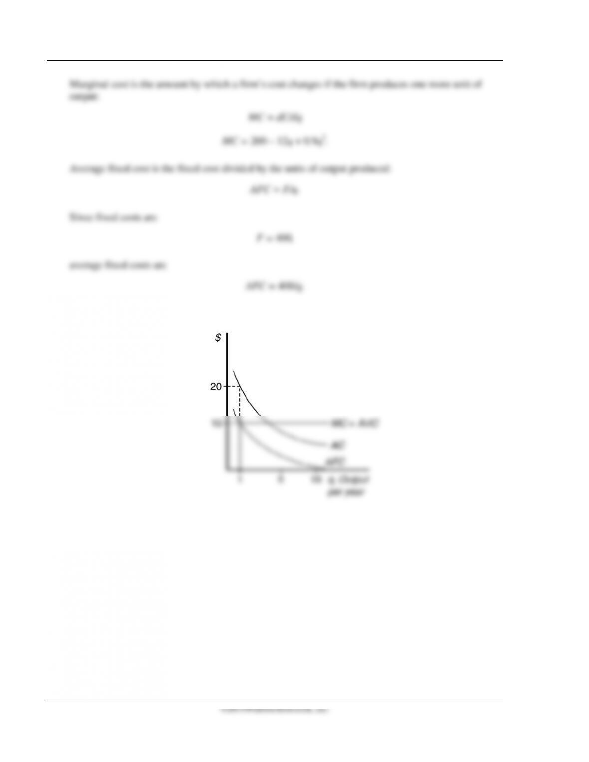
2.1 A fixed cost is a production expense that does not vary with output. $400 does not vary with output
(q) and is a fixed cost:
F = 400.
Average variable cost is the variable cost divided by the units of output produced:
AVC = VC/q.
136 Perloff • Microeconomics: Theory and Applications with Calculus, Third Edition
©2014 Pearson Education, Inc.
Marginal cost is the amount by which a firm’s cost changes if the firm produces one more unit of
output:
MC = dC/dq
MC = 200 – 12q + 0.9q2.
Average fixed cost is the fixed cost divided by the units of output produced:
AFC = F/q.
Since fixed costs are
F = 400,
average fixed costs are
AFC = 400/q.
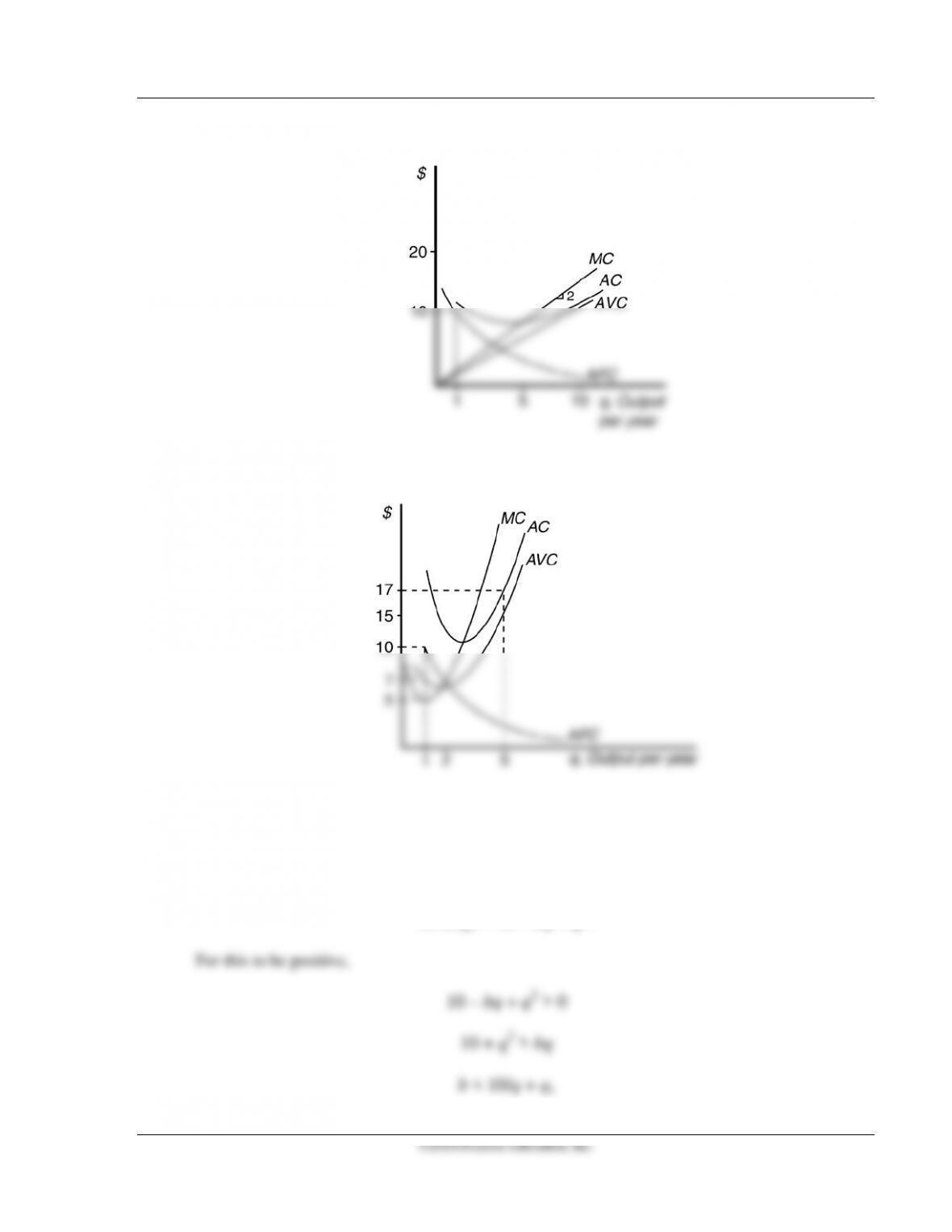
2.2 a. AFC = 10/q. MC = 10. AVC = 10. AC = 10/q + 10.
Chapter 7 Costs 137
b. AFC = 10/q. MC = 2q. AVC = q. AC = 10/q + q. See the figure below.
c. AFC = 10/q. MC = 10 − 8q + 3q2. AVC = 10 − 4q + q2. AC = 10/q + 10 − 4q + q2. See the figure
below.
2.3 a. Variable cost is
VC(q) = 10q – bq2 + q3.
Average variable cost is
138 Perloff • Microeconomics: Theory and Applications with Calculus, Third Edition
©2014 Pearson Education, Inc.
b. The average cost curve is U-shaped. AC is minimized at dAC/dq = −Fq−2 − b + 2q = 0.
c. MC crosses AC when the functions are equal. MC = AC where 10 − 2bq + 3q2 = F/q + 10 − bq + q2.
MC = AVC where 10 − 2bq + 3q2 = 10
−
bq + q2, or where q = b/2.
d. AVC is minimized where dAVC/dq = 0.
dAVC/dq = – b + 2q = 0
or b = 2q
MC = AVC
where
10 − 2bq + 3q2 = 10 − bq + q2.
Substituting 2q for b on both sides yields
10 − q2 = 10 − q2
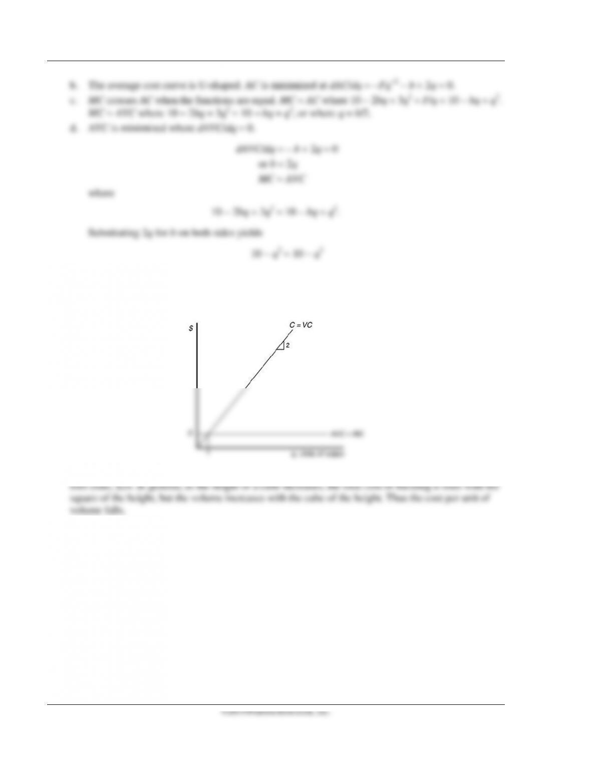
2.4 Let q equal the number of offices cleaned per hour. Then C = 2q (15 minutes of labor is required per
office). Variable cost is also 2q because there are no fixed costs. Average variable cost and marginal
cost are $2. See figure below.
2.5 The total cost of building a 1–cubic-foot crate is $6. It costs four times as much to build an 8-cubic-
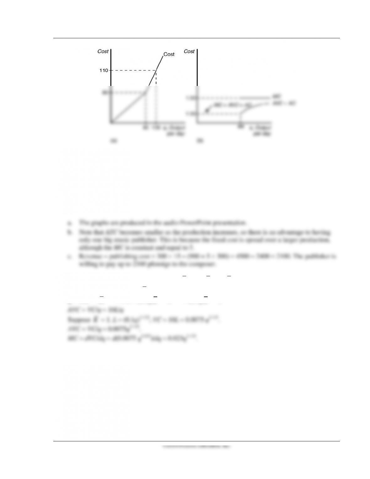
2.6 C = q, MC = AVC = AC = 1 for q less than or equal to 80 per day. C = 80 + 1.5 (q − 80) = 1.5q − 40,
MC = 1.5, AVC = AC = 1.5 − 40/q for all q greater than 80 per day. See figures below.
Chapter 7 Costs 139
©2014 Pearson Education, Inc.
2.7 TC = 900 + 5q,
AFC = 900/q,
AVC = 5,
ATC = 900/q + 5,
MC = 5.
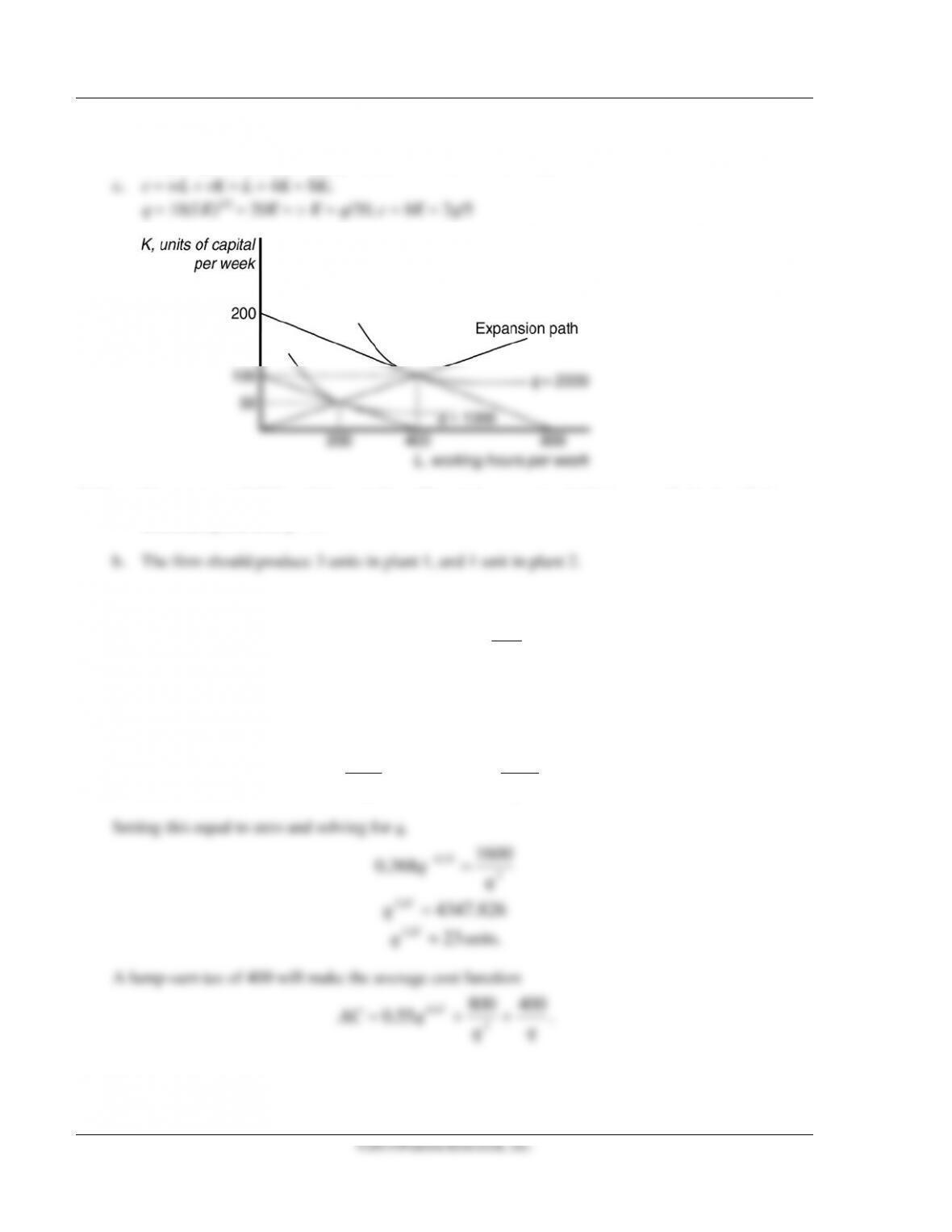
2.8 In the short run, suppose capital is fixed at
.K
F = r
K
= 20
K
; VC = wL = 10L.
Total cost C = F + VC = 20
K
+ 10L.
.K
K
K
−0.56)1/0.32 = (0.1q
−0.56)3.125
K
140 Perloff • Microeconomics: Theory and Applications with Calculus, Third Edition
2.9 a. See figure below.
b. MPL/MPK = (1/2q/L)/(1/2q/K) = K/L = w/r = 1/4 = > L = 4K;
2.10 a. You must set dAC/dq = 0 for each firm. The minimum point of AC1 is at q = 2. At plant 2, the
minimum point is at q = 1.
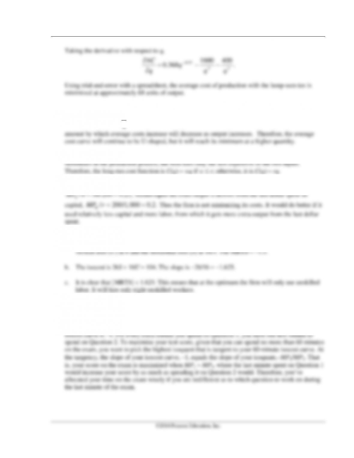
2.11 Average cost is the total cost divided by the units of output produced:
2
67.0
800
55.0 q
qAC +=
.
To find the quantity at which average cost is minimized, take the derivative of the average cost
function with respect to q and solve for q. The derivative of the average cost function with respect to
q is
3
33.0
1600
368.0 q
q
q
AC −=
∂
∂
−
.
q
q
2
Chapter 7 Costs 141
©2014 Pearson Education, Inc.
Taking the derivative with respect to q,
23
33.0
4001600
368.0 qq
q
q
AC −−=
∂
∂
−
.
Using trial–and-error with a spreadsheet, the average cost of production with the lump-sum tax is
minimized at approximately 68 units of output.
2.12 A lump-sum tax of t will increases the total cost of production by t. This will increase the average
cost of production by
q
t
, raising the average cost of production at every output level. However, the
3.1 Let w be the cost of a unit of L and r be the cost of a unit of K. Because the two inputs are perfect
3.2 If the firm were minimizing its cost, the extra output it gets from the last dollar spent on labor,
/ 50/200 0.25,
L
MP w = =
should equal the extra output it derives from the last dollar spent on
capital,
/ 200/1,000 0.2.
K
MP r = =
Thus the firm is not minimizing its costs. It would do better if it
used relatively less capital and more labor, from which it gets more extra output from the last dollar
spent.
3.3 a. The equation of isoquant is (6/8)S + (4/8)U = 4 → 3S + 2U = 16. This equation implies that
S and U are perfect substitutes. The isoquant is a negatively sloped straight line that hits the
3.4 You produce your output, exam points, using as inputs the time spent on Question 1, t1, and the time
spent on Question 2, t2. If you have diminishing marginal returns to extra time on each problem, your
isoquants have the usual shapes: They curve away from the origin. You face a constraint that you
may spend no more than 60 minutes on the two questions: 60 = t1 + t2. The slope of the 60-minute