978-0133019933 Chapter 7 Lecture Note

Unlock access to all the studying documents.

View Full Document

126

Chapter 7

Costs



Chapter Outline

7.1 Measuring Costs

Opportunity Costs

Application: The Opportunity Cost of an MBA

Solved Problem 7.1

Capital Costs

Sunk Costs

7.2 Short-Run Costs

Short-Run Cost Measures

Fixed Cost, Variable Cost, and Total Cost

Marginal Cost

Average Cost

Solved Problem 7.2

Short-Run Cost Curves

Production Functions and the Shapes of Cost Curves

Shape of the Marginal Cost Curve

Shape of the Average Cost Curve

Application: Short-Run Cost Curves for a Japanese Beer Manufacturer

Effects of Taxes on Costs

Short-Run Cost Summary

7.3 Long-Run Costs

Input Choice

Isocost Line

Minimizing Cost

Solved Problem 7.3

Using Calculus to Minimize Cost

Solved Problem 7.4

Maximizing Output

Factor Price Changes

How Long-Run Cost Varies with Output

Expansion Path

Chapter 7 Costs 127

Solved Problem 7.5

Long-Run Cost Function

Solved Problem 7.6

The Shape of Long-Run Cost Curves

Application: Small is Beautiful

Estimating Cost Curves Versus Introspection

7.4 Lower Costs in the Long Run

Long-Run Average Cost as the Envelope of Short–Run Average Cost Curves

Application: Choosing an Ink-Jet or Laser Printer

Short-Run and Long-Run Expansion Paths

How Learning by Doing Lowers Costs

Application: Learning by Drilling

7.5 Cost of Producing Multiple Goods

Application: Economies of Scope



Teaching Tips

The material in Chapter 7 is undoubtedly some of the most important in the entire text. If students are to

have any significant level of understanding of how firms make production decisions when faced with

various industry structures and levels of market power, they must have a sound understanding of cost.

You might begin by asking the class for the kinds of costs that firms must consider. You are likely to

get most or all of the private, explicit costs—labor, materials, and capital—but you may or may not get

suggestions of opportunity costs and social costs. Once you have completed a list, you can distinguish

between cost types and discuss the importance of measuring cost as opportunity costs. You may want to

take some time to discuss externalities and give some examples of firms’ attempts to internalize them (and

why they would do so), such as the production of dolphin-safe tuna. Finally, some students may question

the lack of attention paid to materials as an input and question the assumption that material use is independent

of the capital–labor mix.

As with the production definitions, you can use a running example of output and cost figures that are

presented in a table and subsequently in graphs. Remind students whenever possible that the information

here is directly related to the production function. The text makes specific note of the shape of the variable

cost curve and its relationship to the diminishing marginal returns to labor. This link is further reinforced

by Equations 7.3 (MC = w/MPL) and 7.4 (AVC = w/APL). Marginal cost and marginal product curves can

be described as inverted images of one another, noting that the characteristic “check–mark” or “fish hook”

shape is always there in one if it is there in the other for any given production function. The same applies

to the average product and average cost curves (as well as their intersection with their respective marginal

curves).

When covering long-run cost, you shouldn’t need to spend too much time on isocost lines, other than to

show the equation for the definition of cost and note the similarity to the budget constraint. The one point

worth emphasizing here is that, unlike the budget constraint in utility maximization, the isocost line is the

objective function rather than the constraint. The comparison of the minimization of cost to the maximization

of utility can be continued throughout the discussion of the Lagrangian technique for solving the constrained

128 Perloff • Microeconomics: Theory and Applications with Calculus, Third Edition

minimization problem. Students will see the similarity with the utility maximization problem but often

fail to realize the subtle differences. Graphically, the solutions appear similar yet the utility maximization

diagram will have several convex indifference curves and a single linear budget constraint. The cost

minimization diagram has a single convex isoquant and several linear isocost lines.

The section on the shape of the long-run cost curves and the relationship between long- and short-run cost

is where you may need to slow down significantly. You may need to spend a good deal of time describing

how long–run cost curves are related to the different short–run curves and presenting a verbal and graphical

depiction of the envelope theorem. If it seems that the class is really struggling with the graphs, keep a set

of correctly drawn graphs that will photocopy and hand them out to the class. That way, students can take

notes right on the handouts. Understanding the relationship between marginal, average, and total curves is

essential from this point onward.

This is a great place to make use of a computer–equipped classroom. By entering a cost function such as

C = 2/3q3 − 12q2 + 90q, which has ranges of increasing and decreasing returns, you can show the total,

average, and marginal cost curves for a typical cost function and discuss points of inflection, intersection,

and the relationship between the curves. If you decide to use this specific function, you will need to compute

values for C, AC, and MC through an output level of 16 to see the curve shapes well.

Section 7.5 introduces scope economies. The presentation in the text is brief and straightforward. You may

choose to introduce more of the technical material associated with scope economies, such as incremental

cost and stand–alone cost, but at the intermediate level, conceptual understanding is most important. You

might begin the discussion by asking the class if they can think of any single–product firms (they frequently

cannot). Ask them why this is so. Although they don’t use the terminology of scope economies, the class

often gives responses that refer to these types of savings. Once you get through the basic terminology,

you can choose several large firms, such as Ford or GE, and ask the class for possible sources of scope

economies. If there is a current merger or buyout in the news, you may want to have the class search

through an article in the Wall Street Journal for mention of savings the firm(s) hopes to generate that

amount to scope economies.



Additional Applications

Economies of Scale and Scope in Teaching

Is it less expensive per head to teach more students—that is, are there scale economies in teaching? Nelson

and Hevert (1992) estimate a short–run cost function for departments at the University of Delaware, where

output is measured as the number of student credit hours.1

We expect short–run scale economies if the fixed costs of administration, physical plant, libraries, and

computer centers are large. If so, the average fixed costs are a major component of average total cost.

Nelson and Hevert (1992) do not find evidence of economies or diseconomies of scale if a department

increases quantity by increasing the number of classes (holding class size fixed). In contrast, they find

substantial economies of scale if output is increased by increasing class size.

What are the implications of these findings for marginal cost? In a lecture class, if enrollment is increased

by 50 percent, holding class size constant, the marginal cost falls by 7 percent for a lower–level

undergraduate course, 22 percent for an upper–level undergraduate course, and 21 percent for a graduate

course. If class size is increased by 50 percent and enrollment is held constant, the corresponding changes

1Randy Nelson, and Kathleen T. Hevert, “Effect of Class Size on Economies of Scale and Marginal Costs in Higher Education,”

Applied Economics, 24(5), May 1992:473–82.

Chapter 7 Costs 129

are 17 percent, 12 percent, and 5 percent. That is, increasing either class size or enrollment lowers marginal

cost.

Cohn, Rhine, and Santos (1989) studied economies of scope in teaching in schools across the country.2

They measure teaching output as the number of undergraduate and graduate full-time enrollments (that is,

they do not control for qualitative differences). They measure research output indirectly using funds raised

for sponsored research (presumably, if more funds are available, more good research is produced). At

public colleges and universities, they find virtually no scope economies (SC = −0.064) at average output

levels. For higher levels of output, however, they do find scope economies. At private schools, they find

economies of scope at average levels of output (SC = 0.179) and much higher levels of scope economies

at larger output levels. These results indicate that it is less expensive to produce large amounts of teaching

and research at the same institution as separate ones. Put differently, teaching and research are complementary.

The cost savings from scope are larger at larger institutions.

1. How might the results in these two studies change if quality of education were introduced as an

additional variable? How might this be accomplished?

2. What do you believe are possible sources of scope economies in education and research? Might they

be more prevalent in some disciplines than others?

Entrée Economics—The Cost of a Meal3

Recently, at an upscale New York restaurant, a patron was served a pork chop that cost the eatery about

$6.25, including the chop, spices, garnish, and assorted vegetables, and sauce. The price? $23.50.

While a nearly 400 percent markup may seem exorbitant, it is commonplace in the restaurant industry.

Even worse is the markup for salmon. Brian Buckley, Director of Management Studies at Peter Kump’s

New York Cooking School, noted that while people believe salmon is an elegant dish, and while some

even have visions of Alaska when ordering, they are actually purchasing farm–raised fish that costs the

restaurant about $2.50 per pound. The resulting markup comes to about 900 percent. Markups vary

substantially from food to food even within the same restaurant. At the Sunset Grille in Nashville, demand

restricts the restaurant’s ability to mark up its best tenderloin, thus the fairly small markup of 200 percent.

However, like many restaurants, the Grille has a target markup of 300 percent. It makes up the difference

on vegetables—both side dishes and vegetarian entrées are marked up by as much as 500 percent.

Why do these markups seem so outrageous? The Wall Street Journal reporter Eileen Daspin observes,

“(T)o be fair, focusing on the cost of a restaurant meal’s raw ingredients is like calculating the value of

a Picasso based on the cost of the paint.” Eating out as opposed to eating the same food at home involves

many other costs, such as labor, capital (including lease payments, which can be extraordinary in popular

downtown locations), and atmosphere. Nevertheless, some restaurants track costs of materials down to

the last pinch of spice. Steve Uliss, chef–partner of Tennessee’s Real Barbecue Real Fast restaurants in

Massachusetts, claims “If someone with a heavy hand is portioning out seven ounces of beans, we check it

out.” In addition, if all of these markups make it seem like the restaurant business is a no–lose proposition,

think again. “According to Dun and Bradstreet, 100 out of every 10,000 U.S. restaurants failed in 1997,”

notes Daspin.

1. Do ingredients represent a variable cost for restaurants? (Can they be substituted with labor or capital?)

2Elchanan Cohn, Sherrie L.W. Rhine, and Maria C. Santos, “Institutions of Higher Education as Multi–product Firms: Economies

of Scale and Scope,” Review of Economics and Statistics, 71(2), May 1989:284–90.

3Based on Daspin, Eileen, “Entrée Economics,” Wall Street Journal, March 10, 2000: W1, W4.

130 Perloff • Microeconomics: Theory and Applications with Calculus, Third Edition

2. If materials represent such a small fraction of total cost, then why would firms bother to look for

employees who are “heavy handed” with the side orders?

Daylight Saving Time4

Daylight Saving Time (DST) begins for most of the United States at 2 A.M. on the second Sunday in

March. Time reverts to standard time at 2 A.M. on the last Sunday of October.

DST—for the United States and its territories—is not observed in Hawaii, American Samoa, Guam, Puerto

Rico, the Virgin Islands, the Eastern Time Zone portion of the state of Indiana, and by most of Arizona

(with the exception of the Navajo Indian Reservation in Arizona). California even asked for federal

“approval” to move to a “year-round” Daylight Saving Time in 2001–2002 because of its energy crisis.

DST is also observed in about 70 countries.

One of the biggest reasons we change our clocks to DST is that it saves energy. Energy use and the

demand for electricity for lighting our homes is directly connected to when we go to bed and when we get

up. Bedtime for most of us is late evening through the year. When we go to bed, we turn off the lights and

television.

In the average home, 25 percent of all the electricity we use is for lighting and small appliances, such as

televisions, VCRs, and stereos. A good percentage of energy consumed by lighting and appliances occurs

in the evening when families are home. By moving the clock ahead one hour, we can cut the amount of

electricity we consume each day.

Studies done in the 1970s by the U.S. Department of Transportation show that we trim the entire country’s

electricity usage by about 1 percent each day with Daylight Saving Time. While the amounts of energy

saved per household are small, added up they can be very large.

1. How does DST change a typical household’s “‘production function”‘ in terms of energy usage?

2. In addition to saving energy, can you think of other potential benefits of DST?



Discussion Questions

1. In the short run, are the following examples of fixed or variable costs?

a. A manufacturing firm builds a new plant.

b. A doctor rents an office on a month-to-month basis.

c. A firm hires an unskilled worker.

d. A firm hires an engineer.

2. When would you expect a production possibility curve to be a straight line, and when would you

expect that it would be bowed out away from the origin?

3. Does cost of production depend on demand for a product?

4. Give examples of firms where the long run is reached within a few weeks. Give other examples of

where the long run takes years to reach.

4Bob Aldrich, “Daylight Saving Time, Its History and Why We Use It,” www.energy.ca.gov, California Energy Commission,

website accessed on April 25, 2005.

Chapter 7 Costs 131

5. Give some examples of joint production where you would expect to see economies of scope, no

economies of scope, and diseconomies of scope. Explain why in each case.

6. Why might labor not be a variable input in a hospital setting (such as an operating room)?



Additional Questions and Problems

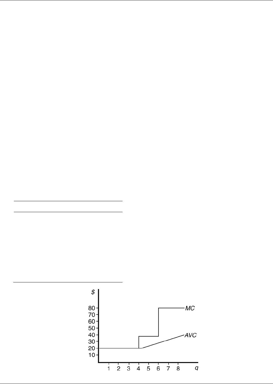
1. Suppose a firm employs labor as its only variable input. All workers are paid $20 per day. Output

per day and variable cost are shown in Table 7.1. Complete the table, showing labor, average

variable cost, and marginal cost for the first eight units of output. Draw a graph showing average

and marginal cost.

Table 7.1

a VC L AVC MC

120

160

240

320

2. True or False, explain your answer. “I paid $25 for the materials to make these flower arrangements,

and sold them at the craft fair for $25, so I just broke even.”

3. Suppose a firm treats capital improvement projects as expenses rather than as investments (which are

amortized). How might this affect the firm’s input usage decisions?

4. Suppose a firm’s average cost curve is described by the equation AC = 2q2 − 16q + 90. At what output

level does the marginal cost curve cross the average cost curve?

5. Explain the relationship between the shape of the marginal cost curve and the marginal product

of labor curve.

6. Suppose the cost of producing milkshakes is C = 0.333Q3 − 3Q2 + 15Q + 50. What is the equation for

marginal cost? At what point is marginal cost minimized?

7. Use a graph to show the marginal cost of attendance for a movie theater (not including the cost of

snacks, just attendance).

8. If input prices are w = 4, and r

1, and q = 4K0.5L0.5, what is the least cost input combination required

to produce 40 units of output? Suppose instead that capital was fixed at 16 units. What would be the

implications for labor usage and total cost?

132 Perloff • Microeconomics: Theory and Applications with Calculus, Third Edition

9. If input prices are w = 3, and r

2, and q = 10KL, what is the least cost input combination required

to produce 60 units of output? How would input usage change if output is increased to 240 units?

Sketch the solutions on a graph.

10. In Question 8, suppose the government, in an effort to increase employment, offers firms in this

industry a $1 per unit subsidy. How would this affect input usage (assume q = 60). How is this likely

to affect employment in the capital goods (K) industry?

11. Two firms currently produce the goods q1 and q2 separately. Their cost functions are C(q1) = 25 + q1,

and C(q2) = 35 + 2q2. By merging, they can produce the two goods jointly with costs described by the

function C(q1, q2) = 45 + q1 + q2. Are there scope economies in this case that would justify the merger?

12. Suppose the production function is Q = a min(K, L), where a is a positive constant, the price of

capital good is $10 per unit, and labor cost is $10 per worker hour. What is the optimal combination

of capital and labor?

13. In Question 12, suppose the production function is Q =

ac min(K, L), where a is a positive constant

and c > 1. The price is of capital good is $10 per unit, and labor cost is $10 per worker hour. What is

the optimal combination of capital and labor? Does the production function have an increasing,

constant, or diminishing return to scale?



Answers to Additional Questions and Problems

1. Table 7.2

q VC L AVC MC

120

160

26.67

240

34.29

8 320 16 40 80