Chapter 6 Firms and Production 114
13. Using what you learn in this chapter, explain why professors often give a short break during a long lecture.
Answers to Additional Questions and Problems
1. In each case, the derivative
∂
Q/
∂
K gives the marginal product of capital MPK.
a. MPK = 1
3. The production function is Q = 2K + L. APL = 2K/L + 1. MPL = 1.
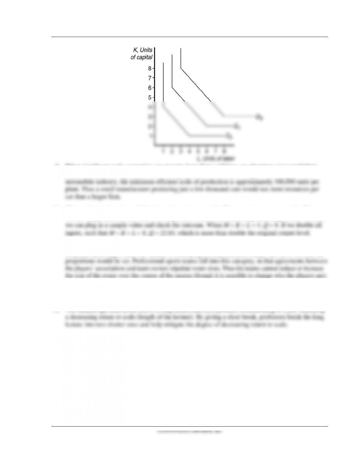
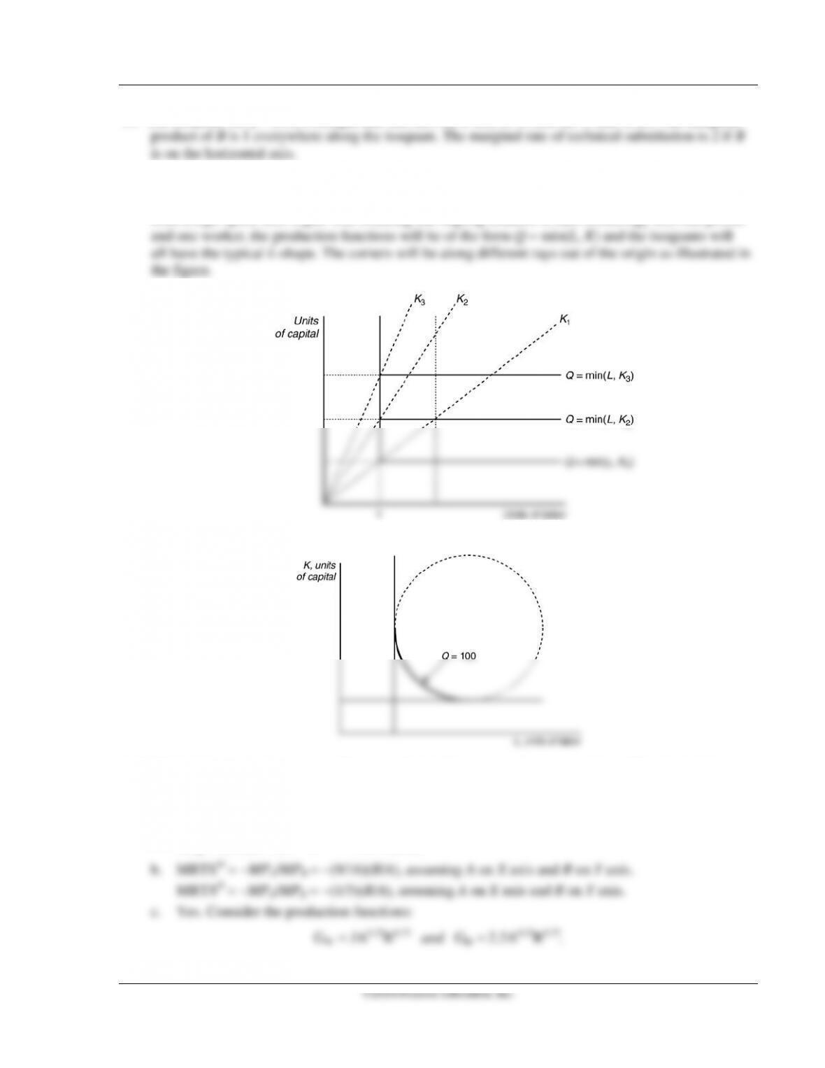
4. The isoquants are “L” shaped, indicating perfect complementarity, and for every doubling of inputs,
output also doubles.
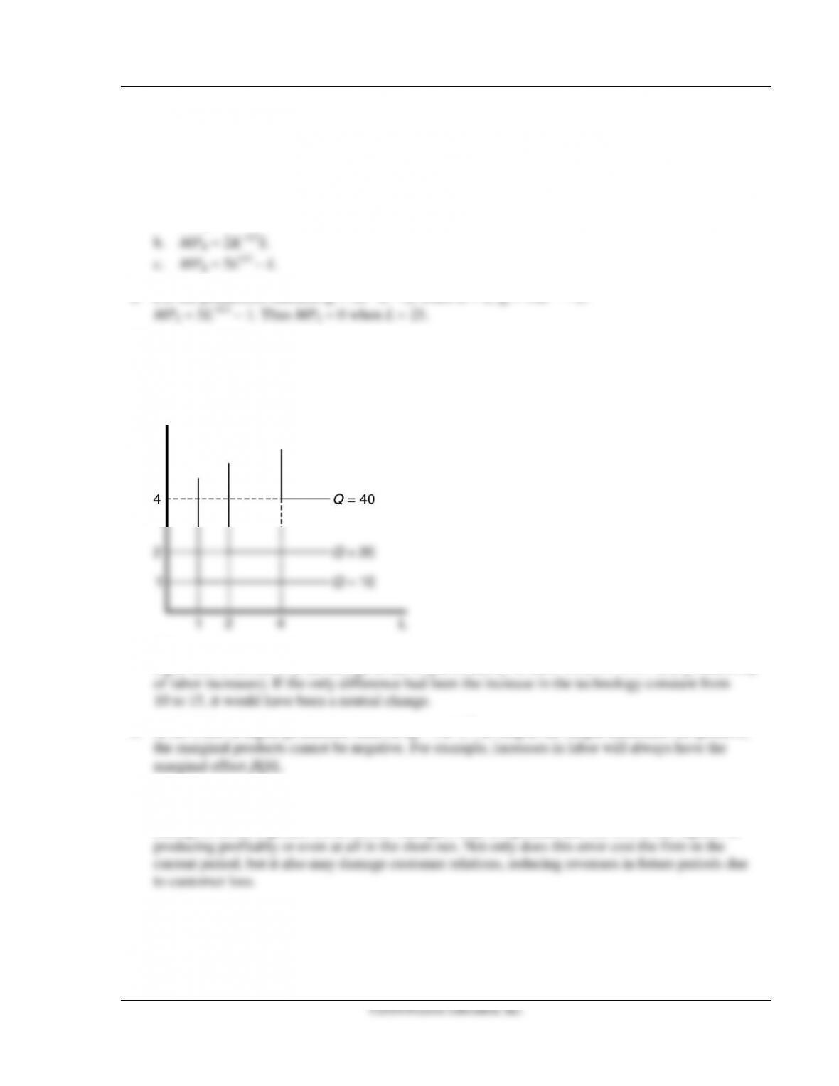
5. This is not a neutral technical change because the marginal productivity of the inputs, and thus the
7. When managers have the incentive to maximize revenue, they may cause the firm to overproduce.
Especially when capital is fixed, there are limits to how much a firm can efficiently produce. In an
8. As long as the input ratio stays with the 4-to–1 limits, the isoquants have a slope of −1. Outside these
limits, they are either vertical or horizontal, indicating that no further substitution is possible.
Chapter 6 Firms and Production 115
©2014 Pearson Education, Inc.
9. When significant scale economies are present, large firms will have an advantage over small firms
because increases in inputs yield more than proportional increases in output. For example, in the
10. This production function exhibits increasing returns to scale. There are two ways to see this. First,
we can simply note that the sum of the exponents exceeds one, indicating increasing returns. Second,
11. When capital and labor are fixed in the short run, production is fixed as well. There would be no
12. The expansion path of this production function is the 45-degree line since the two inputs will always
equal.
Chapter 6 Firms and Production 116
Answers to Exercises in the Text
1.1 Economists usually assume that a firm’s owners try to maximize profit. A firm’s profit is the
1.2 Corporations have limited liability: The personal assets of the corporate owners cannot be taken to
2.1 The more time a firm has to adjust its inputs, the more factors of production it can alter. The short
run is a period of time so brief that at least one factor of production cannot be varied.
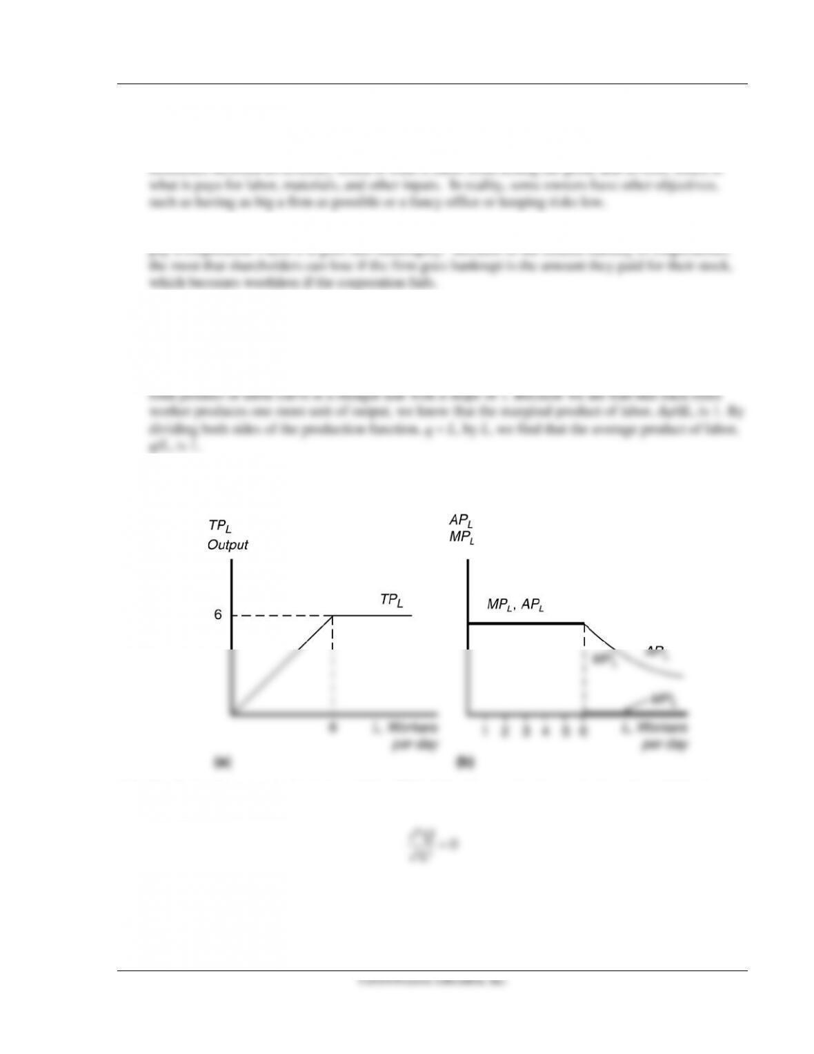
3.1 One worker produces one unit of output, two workers produce two units of output, and n workers
produce n units of output. Thus the total product of labor equals the number of workers: q = L. The
3.2 After the sixth unit, marginal product of labor falls to zero. Total product remains at
six units, and average product of labor falls after the sixth unit.
3.3 No diminishing marginal returns to labor. With K fixed at any level, marginal product of labor is
constant at 10.
2
20
Q
L=
∂
∂
3.4 The production function is
0.75 0.25.qLK=
Chapter 6 Firms and Production 117
©2014 Pearson Education, Inc.
a. As a result, the average product of labor, holding capital fixed at
,
K
is
( )
0.25
0.25
0.25
/ /.
L
AP q L L K K L
−
= = =
b. The marginal product of labor is
( )
0.25
3
4
d /d / .
L
MP q L K L= =
c. APL = (16/L)0.25 = 2L-0.25 . MPL = 0.75(16/L)0.25 = 1.5L-0.25
3.5 The elasticity of output produced with respect to labor is
=L
q
dl
dq
ε
L
L
AP
MP
=
ε
.
4.1 An indifference curve shows all combinations of goods that result in the same level of utility;
an isoquant shows all the combinations of inputs that result in a given level of output.
4.2 If an isoquant were thick, it would imply that the addition of both capital and labor from a point on
Chapter 6 Firms and Production 118
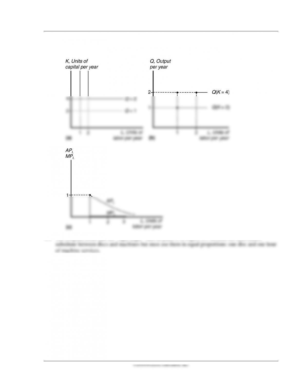
4.3 a. See figure a.
b. See figures b and c.
4.5 Q = L + K.
Chapter 6 Firms and Production 119
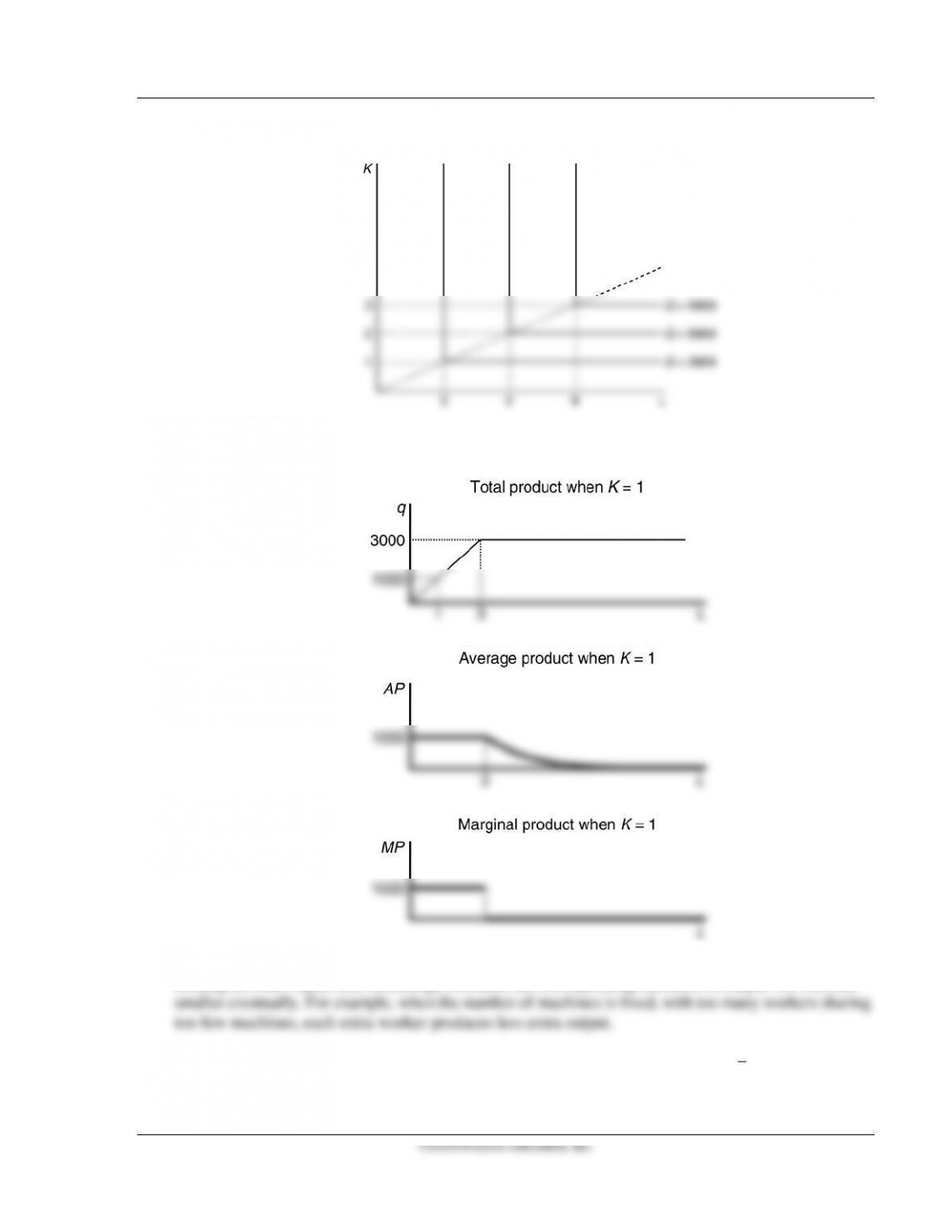
4.6 a. See figure.
b. See figure. Assume the number of copy machines K is fixed at 1. Then production function is Q
= 1000 * min(L, 3). For L ≤ = 3, Q = 1000L; for L > 3, Q = 3000.
4.7 The law of diminishing marginal products indicates that, if a firm keeps increasing one input while
4.8 We know that the marginal rate of technical substitution is
2
3
/.
LK
MRTS MP MP= =
Chapter 6 Firms and Production 120
©2014 Pearson Education, Inc.
4.9 The isoquant for q = 10 is a straight line that hits the B axis at 10 and the G axis at 20. The marginal
product of B is 1 everywhere along the isoquant. The marginal rate of technical substitution is 2 if B
is on the horizontal axis.
4.10 This question will be confusing if students assume all the printers are identical. Each printer is embodied
with a different number of units of capital. For example an all-in–one inkjet copier is very different
4.11 See figure below:
4.12 Michelle’s production process illustrates diminishing marginal returns to labor. This diminishing
return to extra labor may be due to too many workers sharing too few machines or to crowding.
4.13 a.
W
R
MP =
(2.5)(0.64)A0.36R–0.36 = 1.6(A/R)0.36
D
R
MP =
(2.5)(0.75)A0.25R–0.25 = 1.875(A/R)0.25

Chapter 6 Firms and Production 121
These functions have different marginal products but the same MRTS.
4.14 If one divides the production function by
1/
()
ab+
ρ
and also multiplies by this term, one derives the
second expression, where c is the “share” (lies between 0 and 1).
4.15 The marginal rate of technical substitution (MRTS) tells us how many units of capital the firm can
replace with an extra unit of labor while holding output constant. That is, it is the change in capital
relative to the change in labor, and it equals the negative of the ratio of the marginal products:
MRTS =
K
L
MP
MP
dL
dK −=
.
1
−
ρ
K
b
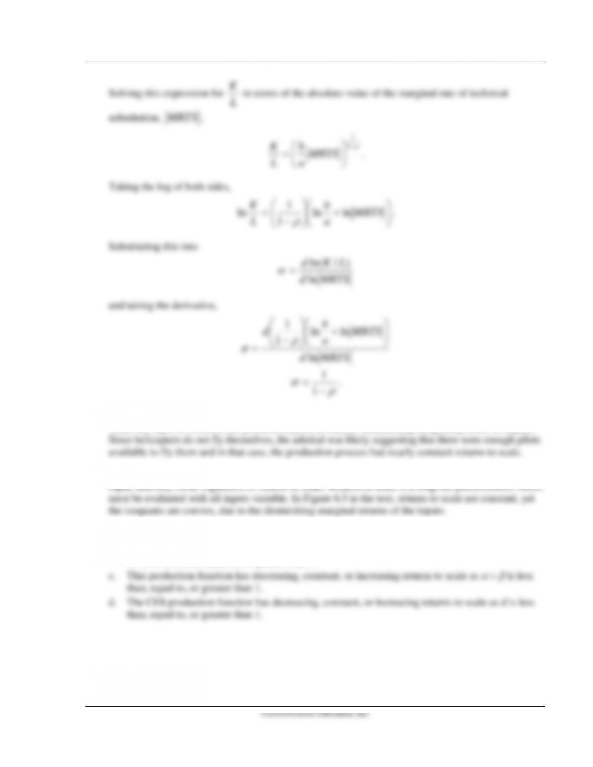
4.16 The elasticity of substitution is the percentage change in the capital–labor ratio divided by the
percentage change in the MRTS:
MRTS
MRTSd
L
K
LKd
)(
)
/(
)/(
=
σ
.
The elasticity of substitution can be written as a logarithmic derivative:
MRTSd
LK
d
ln
)/ln(
=
σ
.
1
−
ρ
K
b
Chapter 6 Firms and Production 122
©2014 Pearson Education, Inc.
Solving this expression for
L
K
in terms of the absolute value of the marginal rate of technical
substitution,
MRTS
,
ρ
−
=
1
1
MRTS
a
b
L
K
.
Taking the log of both sides,
+
−
=MRTS
a
b
L
Klnln
1
1
ln
ρ
.
Substituting this into
MRTSd
LKd
ln
)/ln(
=
σ
and taking the derivative,
MRTSd
MRTS
a
b
d
ln
lnln
1
1
+
−
=
ρ
σ
ρ
σ
−
=1
1
.
5.1 The inputs are helicopters and pilots, the output is delivery of relief. Since the output will not double
5.2 Diminishing marginal returns is a short–run phenomenon, caused by the invariability of the fixed
5.3 a. This production always displays constant return to scale.
b. The Cobb-Douglas production function has decreasing, constant, or increasing returns to scale as
α
+
β
is less than, equal to, or greater than 1.
Chapter 6 Firms and Production 123
5.4 This production function is a Cobb-Douglas. Even though it has three inputs instead of two, the same
5.5 In this context, γ is a scale elasticity because if inputs change by x percent then output increases by
γ percent. This is because
ba
b
a
K
aL
xK
xL
a
q
q)(
)
(
1
2=
q
1
5.6 For Cobb–Douglas production function
Q
=
ALαKβ, if α
+
β
=
1,
the function is CRS, if α + β > 1, the function is IRS, and if α + β < 1, it is DRS. We also know that:
MPL
=
αALα – 1Kβ and MPK
=
βALαKβ – 1.

Chapter 6 Firms and Production 124
5.8 With
γ
= 1,
11
( , ) (, )f xL xK f L K
′′
=
and
22
( , ) (, )f xL xK f L K
′′
=
which implies
11
22
( , ) (, )
( , ) (, )
f xL xK f L K
f xL xK f L K
′′
=
′′
and the MRTS is independent of x.
5.9 If
( , ) (, )f xL xK x f L K=
γ
then differentiating with respect to x yields
12
(, ) (, )Lf xL xK Kf xL xK
′′
+=
1
(, )x f LK
−
γ
γ
Set x = 1 and
12
(, ) (, ) (, ).Lf LK Kf LK f LK
′′
+=
γ
6.1 The technological progress is not neutral. Because of the technology progress, less labor was required
to spin the same amount of cotton in order to produce the same amount of product.
6.2 In the short run, the marginal product of the first few workers will be greater, as they are now able to
produce more than they could with the old machine on a per-person basis. However, given that the
6.3 While this would be true for the productivity of labor at the amount of output observed, it may not be
6.4 The marginal product of labor of Firm 1 is only 90 percent of the marginal product of labor of Firm 2
7.2 Not enough information is given to answer this question. If we assume that Japanese and American
firms have identical production functions and produce using the same ratio of factors during good
Chapter 6 Firms and Production 125
©2014 Pearson Education, Inc.
output during good times (do they hire the same number of extra workers?). As a result, we cannot
predict which country has the higher average product of labor.
7.3 APL = ( + (1 – ))
()
= –APL + MPL
> 0; and if MPL < APL, ()
< 0.