Chapter 5 Consumer Welfare and Policy Analysis 97
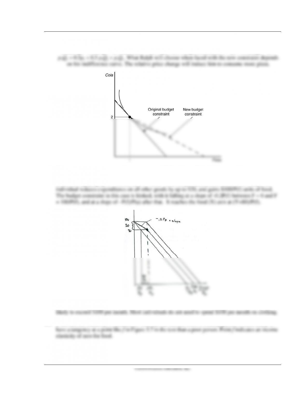
4.2 The original budget constraint is Y = pz Qz + pcQc; normally Ralph buys 1 pizza and 2 colas, which
means Qz = 1 and Qc = 2. Therefore Y = pz + 2pc. New budget constraint: Y = pz + 0.5 pz(Qz − 1) +
4.3 Without any assistance, the individual can buy Y/P(f) of food. With $100 worth of food stamps, the
individual can consume as much as (Y+100)/P(f) of food, and can consume Y/P(a) of all other goods,
4.4 The food stamps provide greater utility than the clothing stamps because expenditures on food are
Chapter 5 Consumer Welfare and Policy Analysis 98
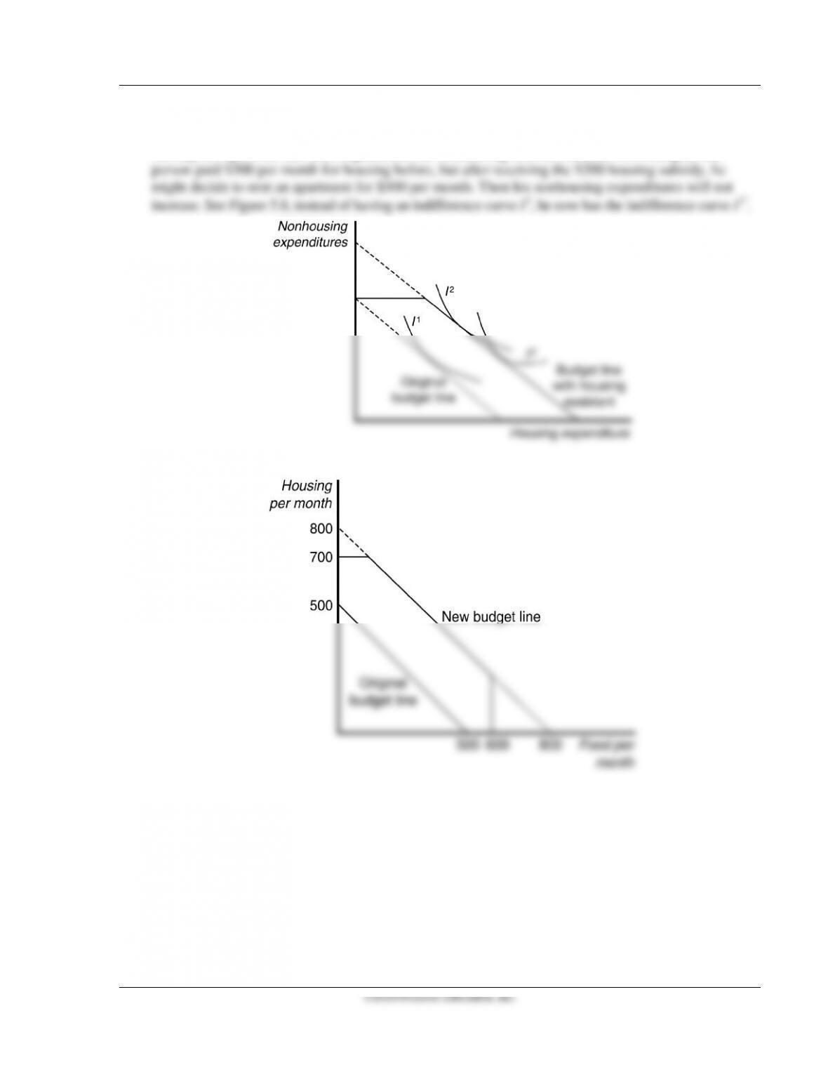
4.6 In normal cases, people will increase their expenditure on nonhousing expenditures with housing
subsidy. However, if people’s tastes (or preference for housing) change after receiving the housing
subsidy, it is possible that their expenditures on nonhousing will not increase. For example, one
4.7 See figure.
Chapter 5 Consumer Welfare and Policy Analysis 99
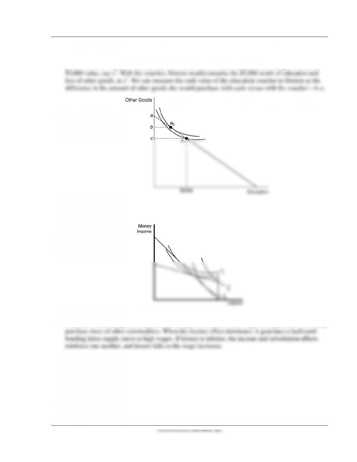
4.8 See figure. Doreen’s budget constraint with the education voucher is kinked, intercepting the vertical
axis at c, while $5,000 cash would cause the constraint to intercept at a. Given that Doreen would
5.1 See figure. Individuals with a high preference for leisure (with indifference curve IB) will accept the
welfare payment. Those with a greater preference for income than leisure (with indifference
curve IA) are likely to turn down the payment.
5.2 Leisure is not a Giffen good. When the wage increases, it increases the opportunity set of the individual.
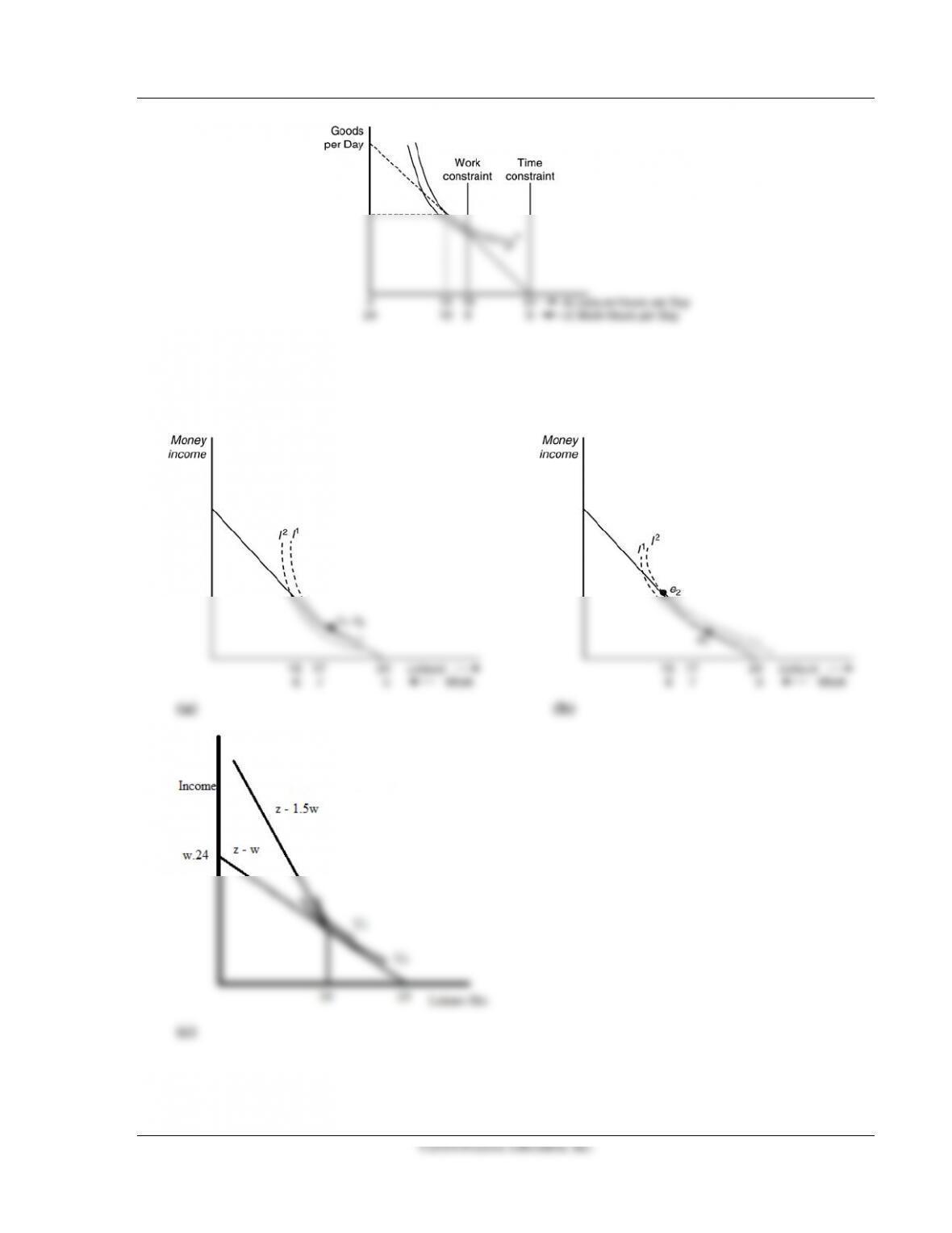
5.3 See figure below. Bessie is unambiguously worse off or she would have chosen the alternative bundle
originally. Because her original optimal bundle lies in the dashed section in the figure, now she has to
choose the corner solution as her optimal bundle.
Chapter 5 Consumer Welfare and Policy Analysis 100
©2014 Pearson Education, Inc.
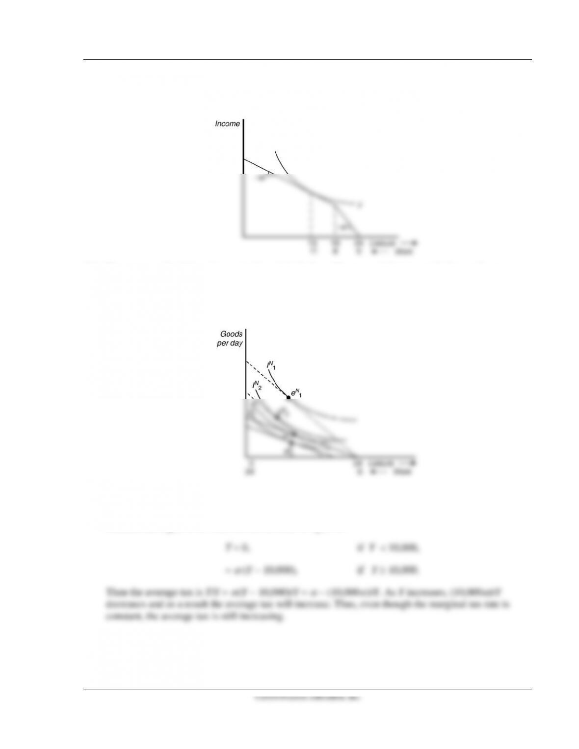
5.4 Whether he decides to work additional hours given the overtime premium depends on his taste for
income versus leisure. Panel (a) shows no additional hours worked, panel (b) shows additional hours
worked. If Roy had originally chosen to work 8 hours per day, he will choose to work more hours
given the overtime wage rate. See panel (c) below.
Chapter 5 Consumer Welfare and Policy Analysis 101
5.5 Jerome’s budget line is kinked at eight hours of work. At that point, the slope of the budget line
increases from −w to −w*. If the job with no restrictions on hours is the higher paying job, Jerome’s
budget constraint would continue at a slope of w > w*, and he would work more hours.
5.6 If we assume that leisure is a normal good, both the noble man and the peasant had to work more
hours with poll tax than when there was no poll tax. Whether a noble man or a peasant worked more
hours depends on the shape of the indifference curves. For example, in the figure below, the noble
man worked fewer hours than the peasant. Indifference curves with greater convexity could illustrate
the opposite case.
5.7 Under progressive income taxes, the marginal tax is higher than the average tax.
5.8 A progressive tax is a tax structure in which the average tax is rising. Assume the marginal tax is
constant and equal to
α
. Then the tax revenue is equal to:
5.9 a. Assume all goods have a unit price. George will work more hours under a lump-sum tax than
under a per-hour tax. A per-hour tax reduces the effective wage but a lump-sum tax does not,

Chapter 5 Consumer Welfare and Policy Analysis 102
©2014 Pearson Education, Inc.
therefore when a lump–sum tax is used, the price for leisure is higher. Hence, George will
consume less leisure but work more hours under a lump-sum tax.
b. The income tax is likely to reduce George’s hours of work more. An income tax reduces the
5.10 As the marginal tax rate on income increases, people substitute away from work due to the pure
substitution effect. However, the income effect can be either positive or negative, so the net effect of
a tax increase is ambiguous. Also, because wage rates differ across countries, the initial level of
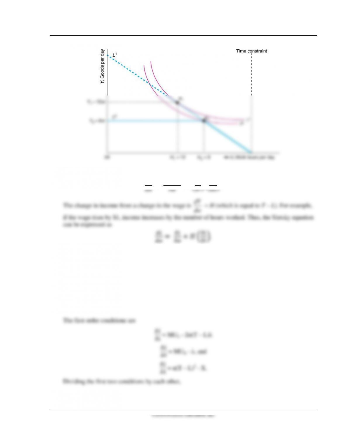
5.11 The figure below shows Julia’s original consumer equilibrium: Originally, Julia’s budget constraint
was a straight line, L1 with a slope of −w, which was tangent to her indifference curve I1 at e1, so she
worked 12 hours a day and consumed Y1 = 12w goods. The maximum–hours restriction creates a kink
in Julia’s new budget constraint, L2. This constraint is the same as L1 up to eight hours of work, and is
horizontal at Y = 8w for more hours of work. The highest indifference curve that touches this
constraint is I2. Because of the restriction on the hours she can work, Julia chooses to work eight
Chapter 5 Consumer Welfare and Policy Analysis 103
©2014 Pearson Education, Inc.
5.12 This is an application of the Slutsky equation. The Slutsky equation is
5.13 Joe’s Lagrangian for utility maximization is
= U(L, X) + λ(w(H)(T – L) – X).
Let L be leisure, X be other consumption, MRS be Joe’s marginal rate of substitution, and MU be
marginal utility. Also, let the price of other consumption be normalized to be $1.00.
Recall that w(H) = αH = α(T – L). Substituting this into the Lagrangian,
= U(L, X) + λ(α(T – L)2 – X).
Chapter 5 Consumer Welfare and Policy Analysis 104
©2014 Pearson Education, Inc.
2( )
L
X
MU TL
MU
αλ
λ
−
=
or
2( )MRS T L
α
= −
.
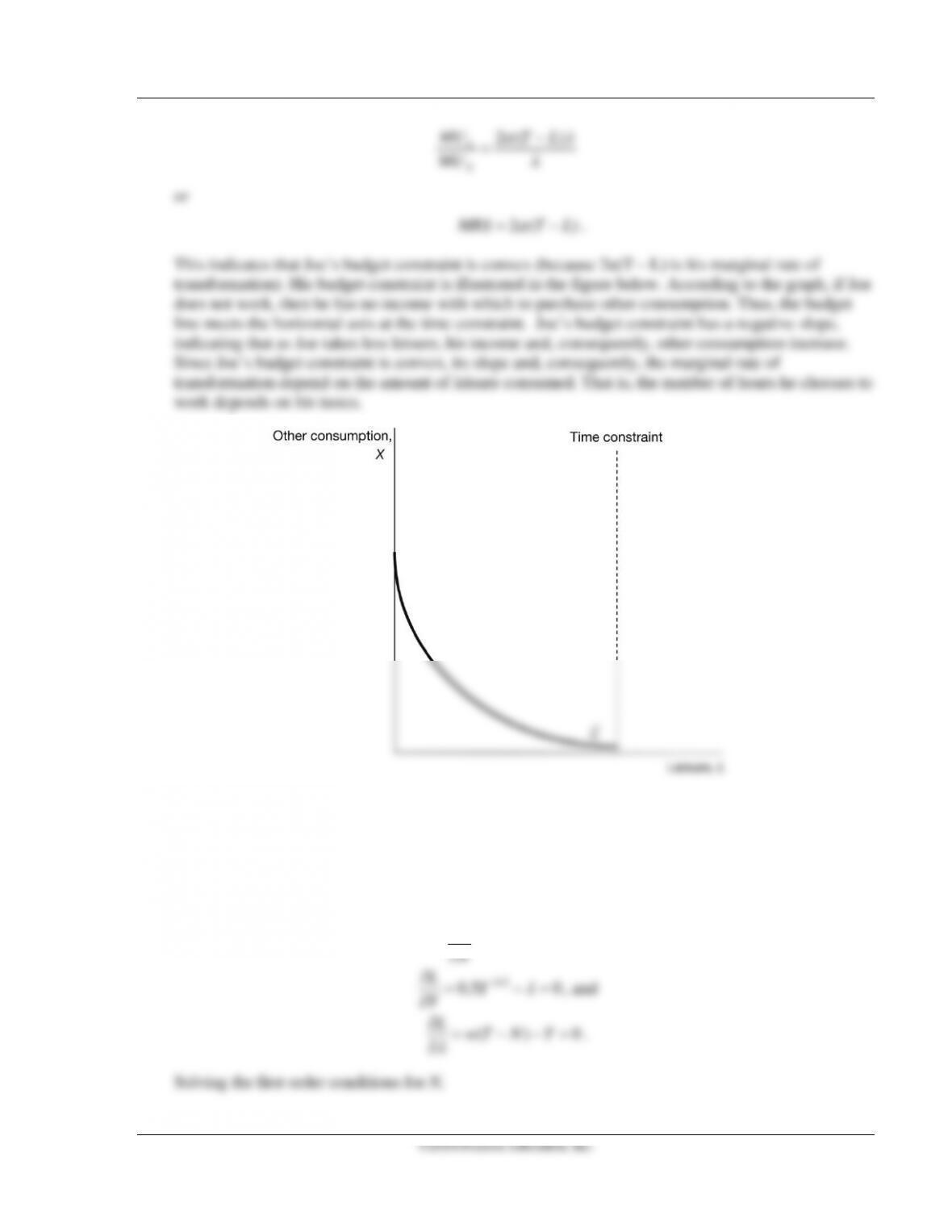
This indicates that Joe’s budget constraint is convex (because 2α(T – L) is his marginal rate of
transformation). His budget constraint is illustrated in the figure below. According to the graph, if Joe
does not work, then he has no income with which to purchase other consumption. Thus, the budget
line meets the horizontal axis at the time constraint. Joe’s budget constraint has a negative slope,
indicating that as Joe takes less leisure, his income and, consequently, other consumption increase.
Since Joe’s budget constraint is convex, its slope and, consequently, the marginal rate of
transformation depend on the amount of leisure consumed. That is, the number of hours he chooses to
work depends on his tastes.
5.14 Sarah’s Lagrangian is
0.5
2 (( ) )L Y N wT N Y
λ
= + + −−
,
where N is leisure, Y is other consumption, w is the wage, and the price of consumption has been
normalized to $1.00. Her first order conditions are
20
Lw
N
λ
∂=−=
∂
,
0.5
0.5 0
LY
Y
λ
−
∂= −=
∂
, and
()0
LwT N Y
λ
∂= − −=
∂
.
Solving the first order conditions for N,
Chapter 5 Consumer Welfare and Policy Analysis 105
©2014 Pearson Education, Inc.
16
w
NT= −
.
Since H = T – N,
16
w
H=
.
This is Sarah’s labor supply function. The slope of Sarah’s labor supply function is
1
16
H
w
∂=
∂
.
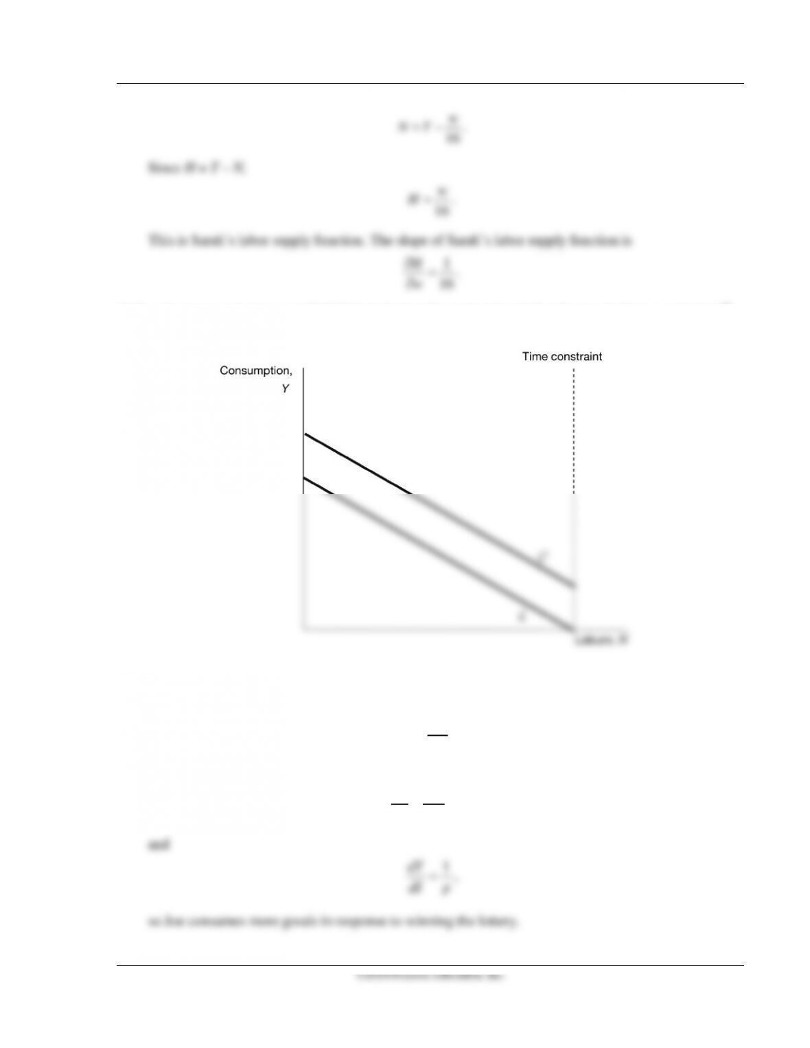
5.15 a. An increase in income will shift Joe’s budget line upward such that the new budget constraint (L2)
will be parallel to the original budget constraint (L1), as illustrated in the figure.
b. Let I be unearned income, w be the wage rate, and T be time. Joe’s demand for leisure is
N =
.
Joe’s demand for leisure is not a function of earned or unearned income. Therefore,
0
dL dH
dI dI
= =
,

Chapter 5 Consumer Welfare and Policy Analysis 107
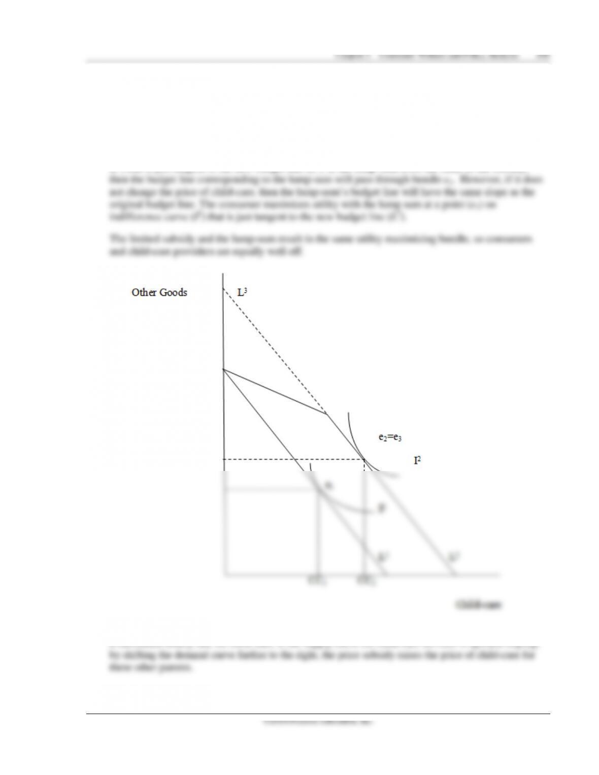
6.3 The government could give a smaller lump-sum subsidy that shifts the LLS curve down so that it is
parallel to the original curve but tangent to indifference curve I2. This tangency point is to the left of
6.4 Limiting the amount of the subsidy decreases utility from the child-care subsidy programs, as long as
the limitation is binding (restricts to less than would have been chosen otherwise). Parents are still
better off with a lump–sum payment.