978-0133019933 Chapter 5 Lecture Note

Unlock access to all the studying documents.

View Full Document

Chapter 5

Consumer Welfare and Policy Analysis



Chapter Outline

5.1 Consumer Welfare

Willingness to Pay

Consumer Surplus

Measuring Consumer Surplus

Application: Willingness to Pay and Consumer Surplus on eBay

Effect of a Price Change on Consumer Surplus

Solved Problem 5.1

5.2 Expenditure Function and Consumer Welfare

Indifference Curve Analysis

Compensating Variation

Equivalent Variation

Application: Compensating Variation and Equivalent Variation for the Internet

Comparing the Three Welfare Measures

An Example

Differences Between the Three Measures

Solved Problem 5.2

5.3 Market Consumer Surplus

Loss of Market Consumer Surplus from a Higher Price

Markets in Which Consumer Surplus Losses Are Large

5.4 Effects of Government Policies on Consumer Welfare

Quotas

Application: Water Quota

Food Stamps

Application: Food Stamps Versus Cash

5.5 Deriving Labor Supply Curves

Labor-Leisure Choice

Solved Problem 5.3

Income and Substitution Effects

Solved Problem 5.4

Chapter 5 Consumer Welfare and Policy Analysis 84

Shape of the Labor Supply Curve

Application: Working After Winning the Lottery

Income Tax Rates and the Labor Supply Curve



Teaching Tips

The material in Chapter 5 introduces the concept of consumer welfare and illustrates the concept using

some applications of government policies that alter the equilibrium and so also change overall welfare.

From the consumer standpoint, you might want to emphasize the difference between the marginal utility,

average utility, and total utility. Students should understand that statements such as I bought these ten candy

bars for $1 each because that’s how much each is worth to me are incorrect. By spending the $10 on the

candy, they reveal that the last candy bar is worth $1 to them; the previous units are worth more, and the

difference is consumer surplus. Not all students will have been exposed to integrals in the introductory

calculus class, so this may need explaining in more detail.

Students are often confused by the difference between compensating and equivalent variation, and even

those that grasp the concept often calculate the wrong one. It is useful to show the similarity between the

CV and the Hicksian decomposition.

The inclusion of the labor supply curve and the labor leisure trade-off in this chapter is another good way

to make the point of the importance of the substitution and income effects. Although it has been extended

and refined in recent years by the inclusion of home production effects, Ashenfelter and Heckman’s paper

(Econometrica, January 1974) on the income and substitution effects of family income is a nice empirical

test of this concept. Briefly, they found that women treat increases in their husband’s income as a pure

income effect (i.e., they “purchase” more leisure by reducing work hours), but husbands do not react to an

increase in their wife’s income (indicating an income effect of zero). Students are likely to have their own

opinions on the validity of this result in today’s labor market, which can lead to a lively discussion.

The effect of income taxes on labor supply is also a good discussion topic. The text describes the attempts

by the Kennedy, Reagan, and George W. Bush administrations to increase both work effort and tax

receipts by decreasing marginal tax rates at the highest levels. If there is time, you might point out the

normative nature of “fair” marginal tax rates, and that while a primary issue for individuals is fairness,

another important aspect of the setting of tax rates is how they may affect work effort and thus revenues.

It may be the case that in order to construct tax proportions that the majority feels is fair, rates would have

to be higher than another scheme judged to be almost as fair but with lower rates and greater work effort.

As an extension of this section, you may want to discuss in class or assign as homework Question 7 in

the Additional Questions and Problems section later in this chapter. This question requires the students to

construct a piece–wise linear budget line due to changes in the marginal tax rate as hours worked increases.



Additional Applications

American Quota Hurts Ukrainian Firms

Since the breakup of the Soviet Union, the U.S. government has lectured the Ukrainian government on the

virtues of a market economy and provided foreign aid ($700 million was pledged in 1994). The U.S.

import policy, however, undermined the Ukrainian transition to a market economy.

Chapter 5 Consumer Welfare and Policy Analysis 85

Several factories in Ukraine turned out stylish, well-made women’s woolen coats, which they shipped

to the United States for about $212 per dozen, and which retailed for between $89 and $139 each.1

The importing of coats from Ukraine, at $30 million per year, was a very small amount of America’s

annual imports of $30 billion. Shipments, however, were increasing so that, by 1994, Ukraine’s coat

exports to the United States exceeded those from all countries but the Dominican Republic and Guatemala.

Under the Caribbean Basin Initiative, the Dominican Republic and Guatemala do not face quotas on

women’s coats. Ukraine was not as lucky.

The increase in Ukrainian imports apparently upset American coat makers in Maine and elsewhere. Senator

George Mitchell of Maine and the Department of Commerce called for a quota, which was applied in

November 1994, because the imports were disruptive to the American women’s clothing manufacturing

industry. This quota was in addition to the tariff of 21.5 percent on wool coat imports. The quota of about

one million coats in 1995 was about half the orders the Ukrainian coat industry had received from

importers by the end of 1994. Indeed, Lou Levy and Sons, a Seventh Avenue coat company, alone

imported one million coats in 1994.

Textiles and apparel are among the most protected sectors of trade in most nations. The GATT, however,

eliminates most of these curbs. Unfortunately, that relief was too late for many Ukrainian workers and factories.

Even the most modern Ukrainian factory laid off one third of its work force after the announcement of the

quota.

1. Why wouldn’t coat buyers pay to have a lobbyist work to defeat this legislation?

2. Might the law have been written differently if a U.S. firm had owned the factory in Ukraine?

Job Sharing May Help Workers to Maximize Utility

The model of labor supply presented in the chapter assumes that workers are free to choose the number of

hours that they work. However, in many occupations, employers typically do not offer part-time work, and

workers are constrained to full-time work. For workers who would choose to work any number of hours

per week other than 40, this alters their utility-maximizing choice of hours and so reduces utility. For

those workers with a high preference for income who would like to work more than 40 hours per week,

they may be able to increase their income by working part-time at a second job. However, for those

employees who would like to work less than 40 hours per week, they could face the choice of working more

than they would like, or not at all. Job sharing is a relatively recent labor market innovation that can provide

a solution. In job sharing, two employees work as partners and share a single full–time position. The

employee receives the benefit of knowing that they have full–time coverage (and maybe even better than

full–time coverage if one partner can cover for the other during vacations and sick time), while the employees

receive the benefit of being able to choose fewer hours of labor market participation and can devote more time

to either leisure or work in the home. Partners may be spouses (as sometimes occurs in academia when

spouses with similar training share a single position) or completely unrelated individuals who have

significant at–home responsibilities that make full-time work undesirable. Employers have responded to

the increased demand for shared jobs. USA Today reports that as many as 28 percent of firms offer job

sharing. Those interested in sharing a job can even use Internet search services specifically designed to

match partners.2

1. Use a graph similar to Figure 5.8a in the text to show an individual who is constrained to working

1Jane Perlez, “In Ukraine, a Free Market Lesson Learned Too Well,” New York Times, January 1, 1995 Business Section, 1.

2Jerry Langdon, “Job Sharing Programs on the Upswing,” at http://www.usatoday.com/careers/news/2001–01–26–jobsharing.htm,

and “Job Share Partner Search,” at http://www.womans-work.com/job_share_search.htm. Accessed 1/1/03.

Chapter 5 Consumer Welfare and Policy Analysis 86

40 hours per week but would prefer to work less (i.e., her utility would be higher if they could choose

another point on the budget line with about half as many hours of work).

2. Show how the individual in the graph would benefit from job sharing. It may help to assume that

there are two individuals with the same taste for market work.



Discussion Questions

1. What are the strengths and weaknesses of the measure of welfare used by many economists:

consumer welfare plus producer surplus?

2. Why might a society prefer a government policy that lowers our standard measure of welfare? Give

some examples.

3. Give some examples of products that are likely to have little if any consumer surplus and explain why.

4. Give some examples of products that are likely to have little if any producer surplus and explain why.

5. Should the government try to pick the marginal tax rate so as to maximize government revenue?

6. Suppose that the price of a product that you frequently buy has increased. Explain in words the

difference between compensating variation and equivalent variation. In practice, are consumers ever

compensated for utility losses due to price changes?

7. Deficit reduction in the coming years may imply increases in income tax rates. How is this likely to

impact work effort? What effect will it have on total taxes collected?



Additional Questions and Problems

1. Demand in Market 1 for X is Qd = 80 − p. Demand in Market 2 is Qd = 120 − 2p. At a price of $20,

which has a larger consumer surplus?

2. True or false, explain your answer. I bought three of these (identical) hats because the price was $10

each and that’s how much each is worth to me.

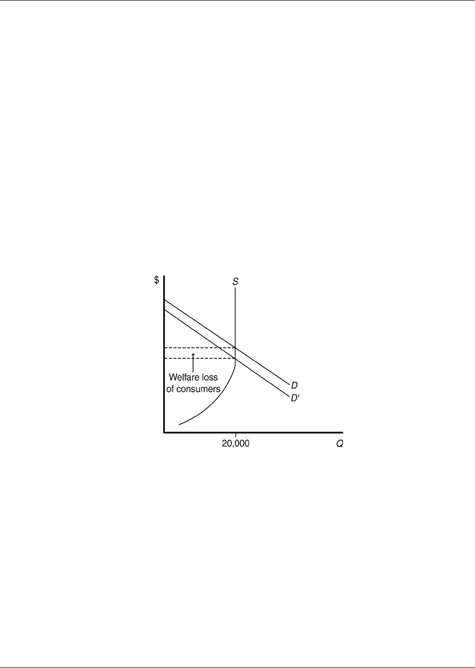
3. Philadelphia Flyers games are frequently sold out, and a waiting list exists for the right to purchase

season tickets. What would be the welfare effects of a $1 tax on tickets? Explain.

4. The NFL’s championship game, called the Super Bowl, is played at a neutral site. Home team fans

must put their names into a lottery for a chance to buy tickets to the game. Winners then purchase

tickets at the stated price. Explain why this allocation mechanism does not maximize total fan welfare.

5. The basic labor supply model presented in this chapter assumes that wage income is untaxed. Suppose

instead that a set of marginal tax rates was imposed such that at a wage of $10/hour, the first 5 hours

of labor were untaxed, the next 10 hours of labor were taxed at a 20 percent rate, and all labor

thereafter was taxed at a 50 percent rate. Show on a graph how this would affect the budget line. How

might this alter work effort?

6. The welfare program was designed to help low-income families. The benefit from this program is

calculated as the fixed percent of the maximum benefit minus family income. Explain why this

design may cause undesirable labor supply effect?

Chapter 5 Consumer Welfare and Policy Analysis 87

7. The conventional welfare program was replaced by the Earned Income Tax Credit program in 1997.

Under the new program, the benefit is calculated as a fixed percent of earnings of low income

families. Explain why this new design helps to encourage labor supply?



Answers to Additional Questions and Problems

1. Surplus in Market 1 is $180 but only $160 in Market 2.

2. This is false unless the consumer’s demand is perfectly elastic. Under normal circumstances, the first

unit is worth more than the marginal unit. If the marginal utility (as revealed by the demand curve)

of the first hat was $20, and the marginal utility of the second hat was $15, and the third hat, $10,

consumer surplus would be $15. If the marginal utility of each hat were $10, the consumer would be

indifferent between purchasing them and not purchasing them.

3. A sold out venue implies that the demand curve crosses the supply curve in its perfectly inelastic

range at current prices, a $1 per seat tax on tickets (which is a small percentage increase for even the

least expensive seats) would reduce consumer welfare by the amount of the tax times the capacity of

the building. If the tax revenues are used for lump-sum grants, the loss becomes a transfer from the

consumers who pay the tax to the consumers who receive the grants. If the building seats 20,000, then

consumer welfare falls by $20,000.

4. The allocation mechanism is inefficient because there is no guarantee that the fans who value the

tickets the most will receive them. Suppose the winning fans may purchase tickets for $100 each. If

a fan who is just willing to pay the $100 receives a ticket, that fan will purchase one, with a net

consumer surplus of $0. If the ticket had instead gone to another fan who values the ticket at $500,

overall welfare increases by $400. The problem is, with a lottery, there is no way to ensure that the

fans who value the tickets most will get one. Thus scalpers emerge and create a secondary market for

resold tickets.