Chapter 4 Demand 71
©2014 Pearson Education, Inc.
=
+
The partial derivative of the demand for q1 with respect to Y is
=
.
Therefore, the income elasticity of demand is
=
1
=1
+
+
= 1
s in the case of the Cobb Douglas utility function, the income elasticity of demand in the case of perfect
complements is 1.
2.6 From Table 4.1(page 102)
=
+
2.7 An Engel curve shows the relationship between the quantity demanded of a single good and income,
holding prices constant. From the Lagrangian for utility maximization,
0.5
1 2 11 2 2
4( ) ( )L q q Y pq pq
λ
= ++ − −
,
the optimal values of good q1 and q2 are
2
2
1
1
2p
qp
=
and
2
12
2
12
(2 )pY p
qpp
−
=
.
These are Sally’s demand functions. Since q1 is not a function of Y, Sally consumes the same amount
of good q1 regardless of income. Solving her demand function for good q2 for Y, her Engel curve is
=
.
(The parenthesis was misplaced. 4 is not squared.)
72 Perloff • Microeconomics: Theory and Applications with Calculus, Third Edition
3.1 The income effect reinforces the substitution effect for normal goods. It partially offsets the substitution
effect for inferior goods. When it more than offsets the substitution effect, it is known as a Giffen good.
3.2 An opera performance must be a normal good for Don because he views the only other good he buys
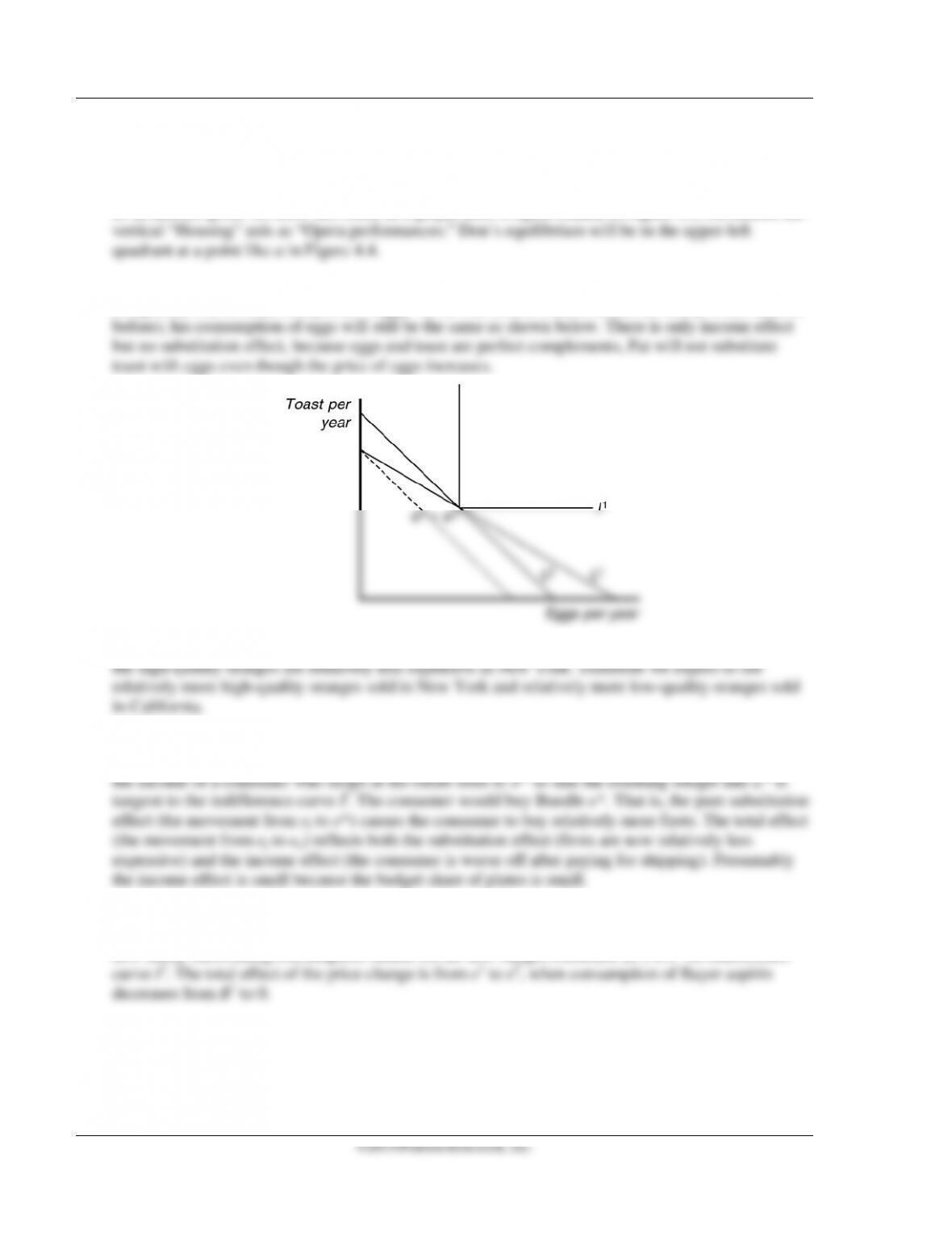
3.3 Eggs and toast are perfect complements. U = min (3Qt, 2Qe). If the price of eggs increases, we
compensate Pat to make him just as “happy” as he was before (which means his utility is the same as
3.4 The low–quality oranges are relatively less expensive in California due to the shipping costs. Likewise,
3.5 On the graph, Lf is the budget line at the factory store and Lo is the constraint at the outlet store. At the
factory store, the consumer maximum occurs at ef on indifference curve If. Suppose that we increase
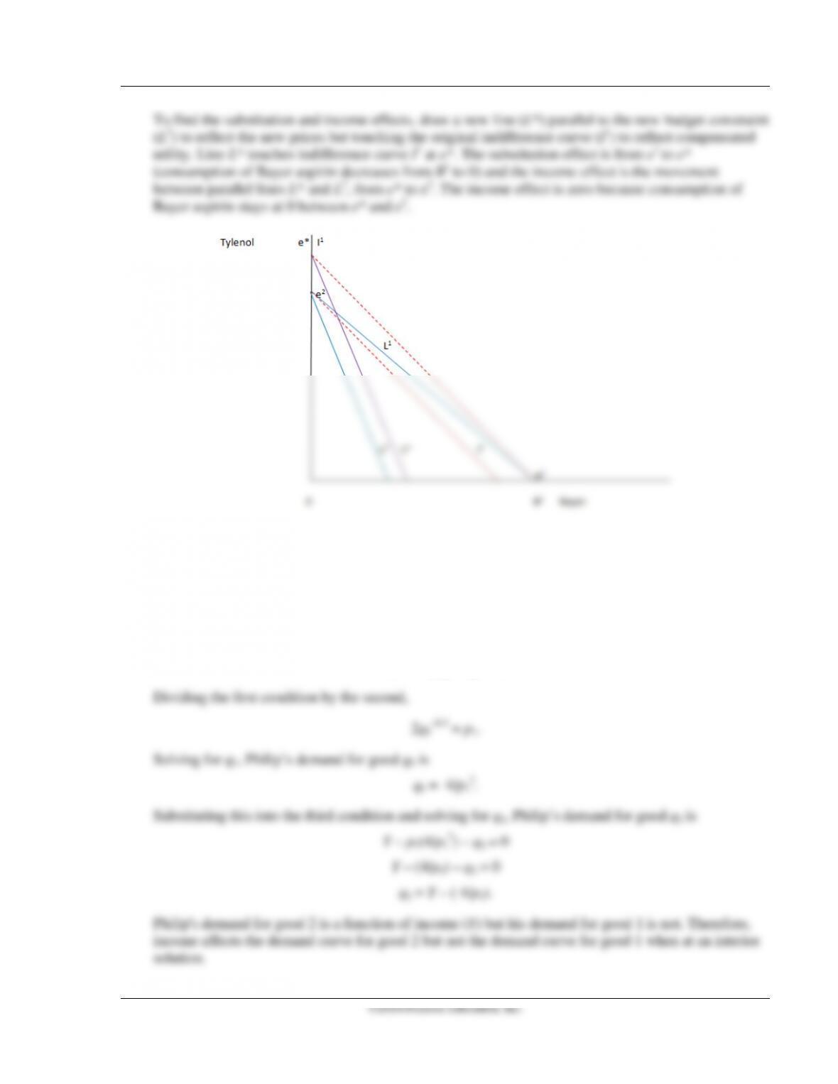
3.6 Initially, when Bayer aspirin is cheaper (on budget line L1), only aspirin is consumed (at e1 on
indifference curve I1). Then, the price of aspirin increases, making Tylenol relatively cheaper. The
Chapter 4 Demand 73
©2014 Pearson Education, Inc.
To find the substitution and income effects, draw a new line (L*) parallel to the new budget constraint
(L2) to reflect the new prices but touching the original indifference curve (I1) to reflect compensated
utility. Line L* touches indifference curve I1 at e*. The substitution effect is from e1 to e*
(consumption of Bayer aspirin decreases from B1 to 0) and the income effect is the movement
between parallel lines L* and L2, from e* to e2. The income effect is zero because consumption of
Bayer aspirin stays at 0 between e* and e2.
3.7 Philip’s Lagrangian is
L: 4q10.5 + q2 + λ(Y – p1q1 – q2). (Hint: p2=1)
The first order conditions are
L1: 2q1–0.5 – p1λ = 0,
L2: 1 – λ = 0, and
L3: Y – p1q1 – q2 = 0.
74 Perloff • Microeconomics: Theory and Applications with Calculus, Third Edition
©2014 Pearson Education, Inc.
The effect of a change in p on the demand for good 1 is
=8
The total effect of a price change (ε) equals the substitution effect (ε*) plus the income effect (–θξ):
ε = ε*– θξ.
Since the demand for good 1 does not depend on income when at an interior optimum, the income
effect is zero, and the total effect equals the substitution effect:
ε = ε*==8
.
3.8 It is impossible for either ice cream or fudge sauce to be a Giffen good. dq/dp is negative for both
members of a perfectly complementary pairing. (Hint: Quotient rule)
3.9 The expenditure function (E) is the relationship showing the minimal expenditures necessary to
achieve a specific utility level for a given set of prices. Since q1 and q2 are perfect complements,
Sylvia will consume them in fixed proportions. So, her uncompensated demand functions are
q1=
2
1
Yp
pj
+
and q2=
2
1
2
Yp
p+
.
3.10 From the Lagrangian for cost minimization,
11 2 2 1 2
( 0.5ln( ) 0.5ln( ))L pq pq U q q
λ
=+ +− −
,
2
2
2
p
p<
3.11 The expenditure function (E) is the relationship showing the minimal expenditures necessary to
achieve a specific utility level for a given set of prices. The expenditure function is the inverse of the
indirect utility function. First, for Sylvan, q1 and q2 are perfect substitutes, so he’ll consume only good
q2 if
2
1
2
p
p<
. So, his uncompensated demand functions if
2
1
2
p
p<
are
q1 =
0
and q2 =
2
Y
p
.
If
2
1
2
p
p>
then
q1 =
1
Y
p
and q2 =
0
.
2
p
76 Perloff • Microeconomics: Theory and Applications with Calculus, Third Edition
©2014 Pearson Education, Inc.
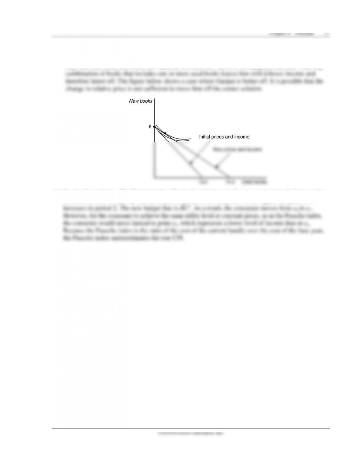
4.2 See figure below. Jean is equally well off at e2 compared to e1. Even if coffee becomes relatively
cheaper, Jean won’t raise her utility by consuming more coffee because cream and coffee are
perfect complements.
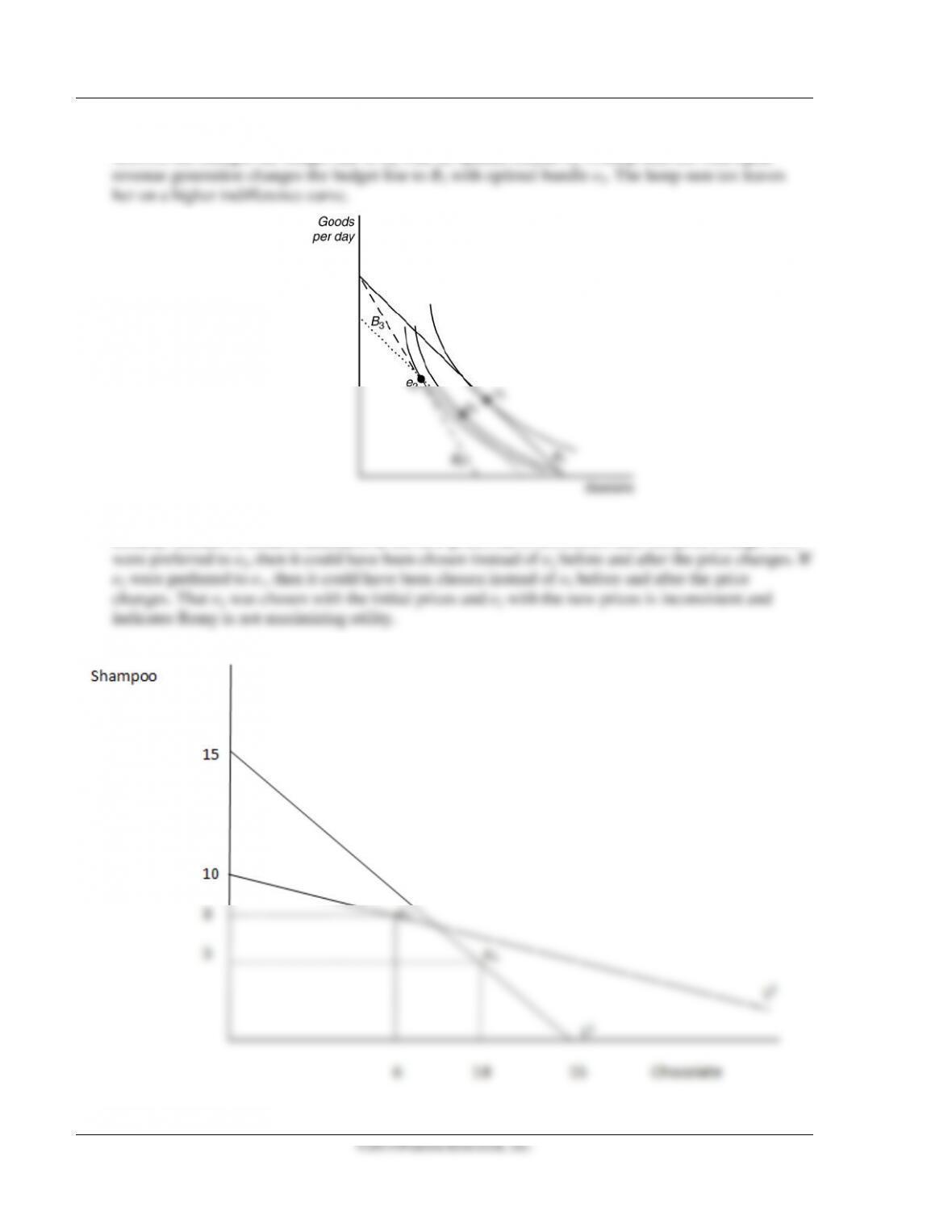
4.3 See figure below. Ann will buy more books and less ice cream this year, and her utility will be better
4.4 The attractive feature of the Big Mac as an indicator of price index is its uniform composition.
78 Perloff • Microeconomics: Theory and Applications with Calculus, Third Edition
4.7 See the figure below. Without the tax Cynthia chooses point e1 on budget constraint B1. An ad
5.1 Remy is not maximizing utility. Bundle e2 was attainable at the initial prices, but it was not chosen

Chapter 4 Demand 79
5.2 Remy is not maximizing utility because the quantities of the goods she consumes move in the same
direction as the price changes.
Given downward-sloping indifference curves, price and quantity must move in opposite directions:
When the price rises, the quantity falls. If so, then the product of the difference in prices multiplied
by the difference in quantities must be nonpositive:
1 21 2
( )( ) 0.
i ii i
p pqq− −≤
5.3 After the income and price change, Felix spends $1,050 on food (from income of $1,200 minus
expenditures of $150 on clothing). At a price of $10 per unit of food, this is 105 units of food. Felix’s
6.1 See the figure below. The company is still paying Alexx to afford the same bundle; however, just like
in the Challenge solution, the original bundle is not optimal, as the relative prices differ in the two
cities.

80 Perloff • Microeconomics: Theory and Applications with Calculus, Third Edition
6.2 Initially, Jim purchases 2000 units of each good. After the move, he purchases 1333.33 units of each
good. To compensate Jim for the move, he needs to receive enough income to continue to purchase
6.3