
Chapter 4 Demand 61
Additional Questions and Problems
1. Suppose the government wants to increase the ability of families to pay for college education. Would
a $500 income tax rebate differ from a $500 tax credit for tuition reimbursement? Explain.
2. True, False or Uncertain; explain your answer. When income rises and the price of x falls, the
consumer will always buy more units of x.
3. Suppose that a consumer’s annual demand for office visits is described by the equation Q = 8 − 0.1p.
If office visits cost $30, and the consumer has no health insurance (i.e., the consumer pays full price),
how many office visits will she make? What is the elasticity of demand for office visits at this point?
Suppose a health insurance plan is instituted that pays for one-third of each office visit. How would
this affect the quantity and the demand elasticity at the new equilibrium?
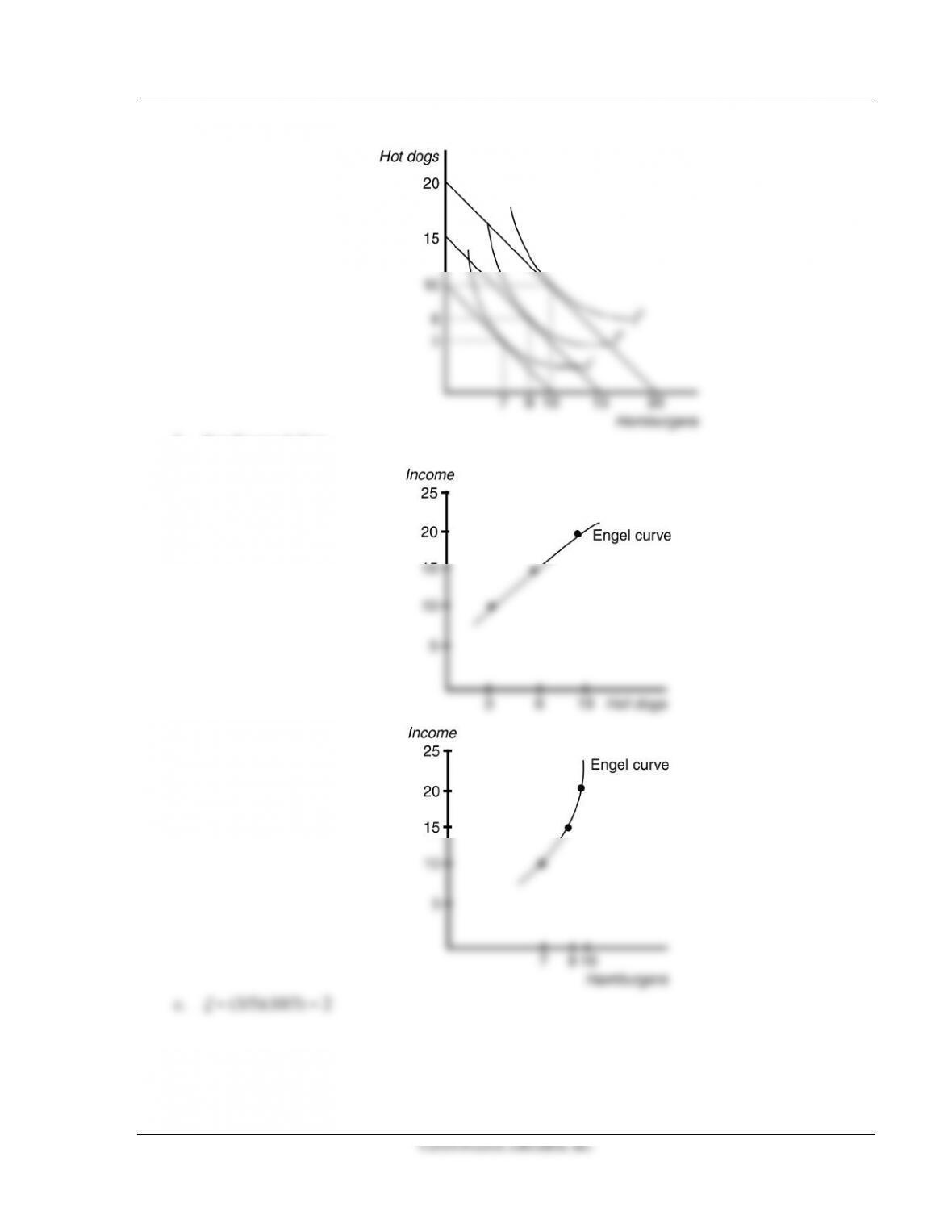
4. A consumer faces prices for hot dogs and hamburgers of $1 each. Consumption of the two
commodities at various weekly income levels are shown below.
a. Use the information to sketch the income consumption curve on a graph.
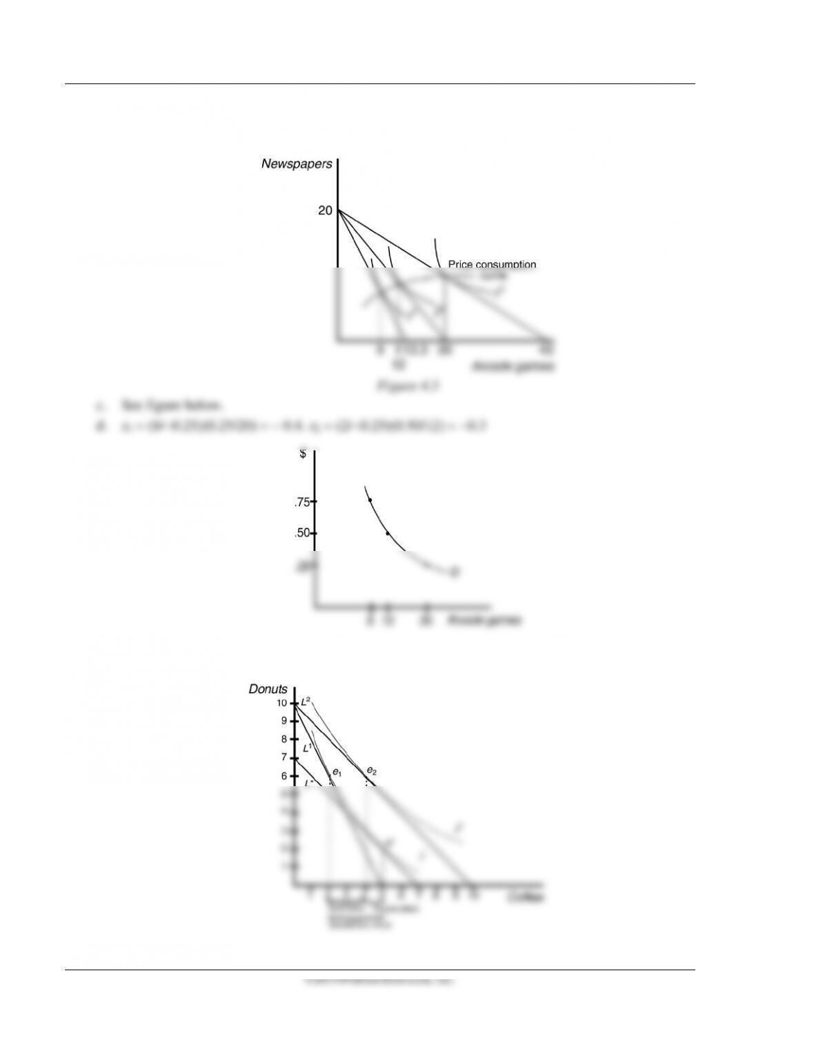
b. Draw the Engel curves for hot dogs and hamburgers.
Income
Hot Dogs
Hamburgers
$10
3
7
15
6
9
20 10 10
c. What is the income elasticity of hot dogs for this consumer as income increases from $10 to $15?
5. Draw a graph with arcade games on the horizontal axis and newspapers on the vertical axis. Joe has
$10 per week to allocate between these commodities. The price of newspapers is $0.50. At the initial
price for arcade games of $0.25, Joe purchases 10 newspapers and plays 20 games. When the price of
games increases to $0.50, Joe purchases 8 newspapers and plays 12 games. When the price of games
increases again to $0.75, Joe buys 5 papers and plays 10 games.
a. Use this information to draw the utility maximizing points on a graph.
b. Draw the price-consumption curve.
c. Draw the individual demand curve for arcade games.
d. Use the information given to calculate Joe’s elasticity of demand for arcade games between
$0.25 and $0.50, and between $0.50 and $0.75.
62 Perloff • Microeconomics: Theory and Applications with Calculus, Third Edition
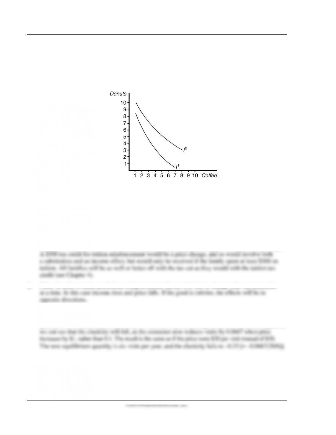
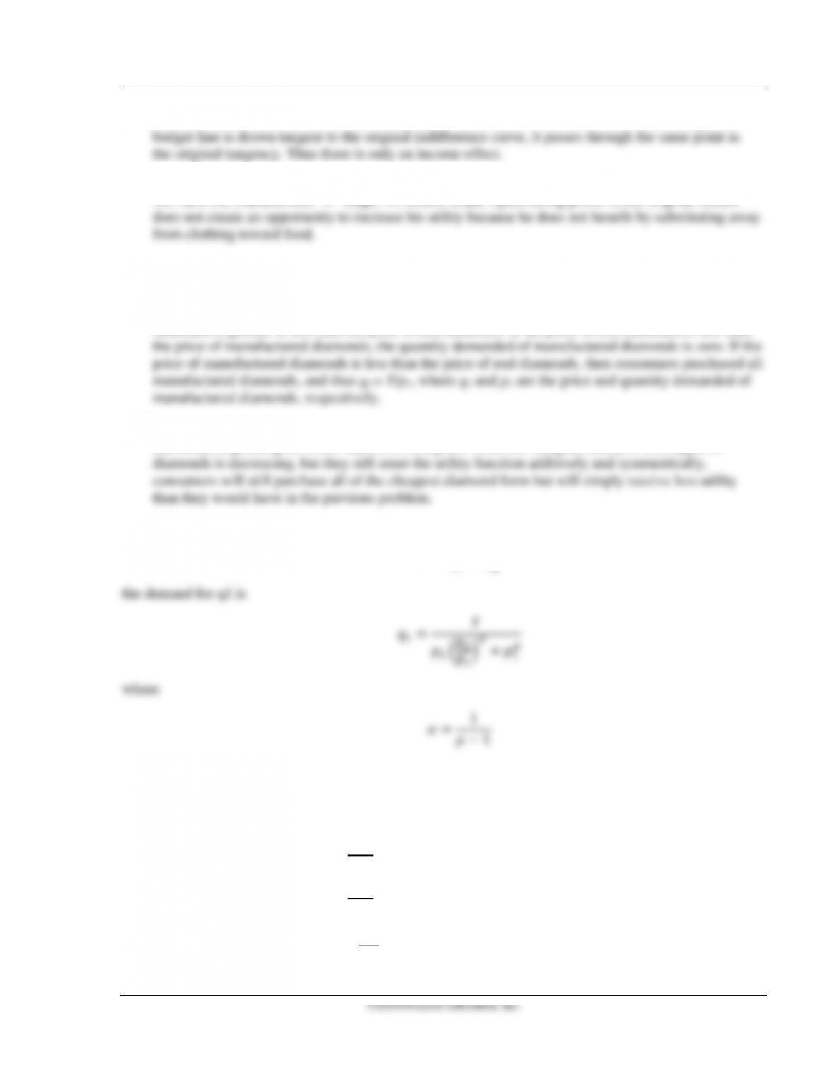
6. Sarah allocates her income of $5.00 between the consumption of donuts and coffee. Her tastes and
preferences are indicated by the indifference curves shown in the figure below. The price of donuts is
$0.50 each. Initially the price of coffee is $1.00 per cup. Subsequently, the price of coffee falls to
$0.50 per cup. On the graph below, show the initial utility maximizing position, the new utility
maximizing position, and separate the income and substitution effects. For Sarah, is coffee a normal
or inferior good?
7. What would the value of the substitution effect be for two goods that are perfect complements? Use
a graph to demonstrate your answer.
8. What happens to the magnitude of the overcompensation due to the use of the CPI in Figure 4.7 in the
text if one views food and clothing as perfect complements?
Answers to Additional Questions and Problems
1. Yes. A $500 reduction in income taxes would represent a pure income effect, providing families with
additional disposable income that could be spent on anything (including, but not necessarily college).
3. If the consumer has no health insurance, she will make five office visits per year, and the elasticity of
demand is −0.6. If an insurance plan covers one-third of the cost of an office visit, the consumer’s
Chapter 4 Demand 63
4. a. See figure below.
b. See figures below.
64 Perloff • Microeconomics: Theory and Applications with Calculus, Third Edition
5. a. See figure below.
b. See figure below.
6. To separate the income and substitution effects, draw the imaginary budget line I*. In this case, because
the income effect partly offsets the substitution effect, coffee is an inferior good. See figure below.
Chapter 4 Demand 65
7. Because the indifference curves are L–shaped, the substitution effect is zero. When the imaginary
8. If the consumer views food and clothing as perfect complements, there is no bias. Indifference curves
Answers to Exercises in the Text
1.1. The demand curve for manufactured diamonds depends in part on whether the price of manufactured
1.2 In the previous problem, consumers would simply purchase all manufactured diamonds or all real
1.3. Answer appears to be referring to an entirely different utility function. Given that
=
+
1.4 a. David’s Lagrangian for utility maximization is
L = 10 q10.25 q20.75 + λ(Y – p q1 q1 – p q2 q2).
The first order conditions are
= 2.5 q1–0.75 q20.75 – p q1λ = 0
= 7.5 q10.25 q2–0.25 – p q2λ = 0
dL
d
λ
= Y – p q1 q1 – p q2 q2 = 0.
66 Perloff • Microeconomics: Theory and Applications with Calculus, Third Edition
©2014 Pearson Education, Inc.
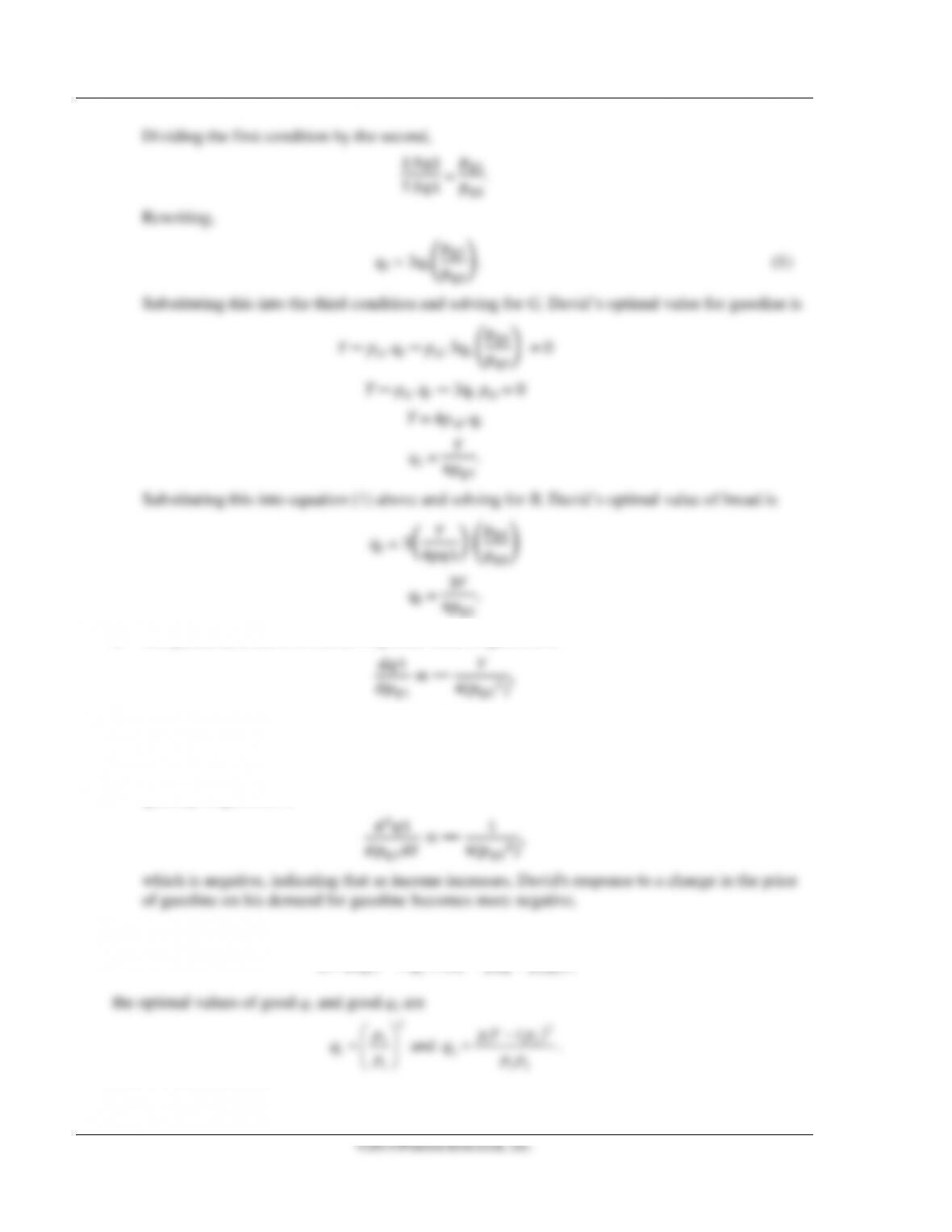
Dividing the first condition by the second,
.
. =
.
Rewriting,
q2 = 3q1
. (1)
Substituting this into the third condition and solving for G, David’s optimal value for gasoline is
Y ─ pq1 q1 ─ pq2 3q1
= 0
Y ─ pq1 q1 ─ 3q1 pq1 = 0
Y = 4p q1 q1
q1 =
.
Substituting this into equation (1) above and solving for B, David’s optimal value of bread is
q2 = 3
q2 =
.
b. The partial derivative of David’s optimal value of gasoline is
which is negative, indicating that David will demand less gasoline w hen the price of gasoline
increases.
c. The partial derivative of the effect of a change in the price of gasoline on David’s optimal
quantity of gasoline is
1.5 From the Lagrangian for utility maximization,
0.5
1 2 11 2 2
2( ) ( )L q q Y pq pq
λ
= ++ − −
,
the optimal values of good q1 and good q2 are
2
2
1
1
p
qp
=
and
2
12
2
12
()pY p
qpp
−
=
.
Chapter 4 Demand 67
These are Philip’s demand functions.
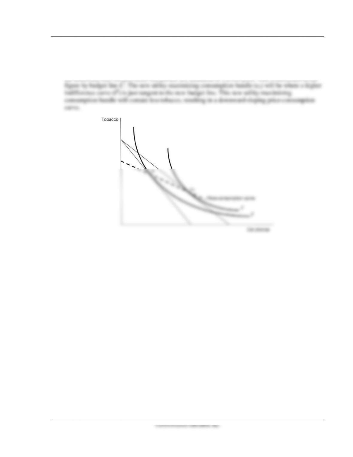
1.6 An individual is initially maximizing utility at consumption bundle e1 on budget line L1, as illustrated
in the figure. When the price of cell phones decreases, the budget constraint will pivot outward along
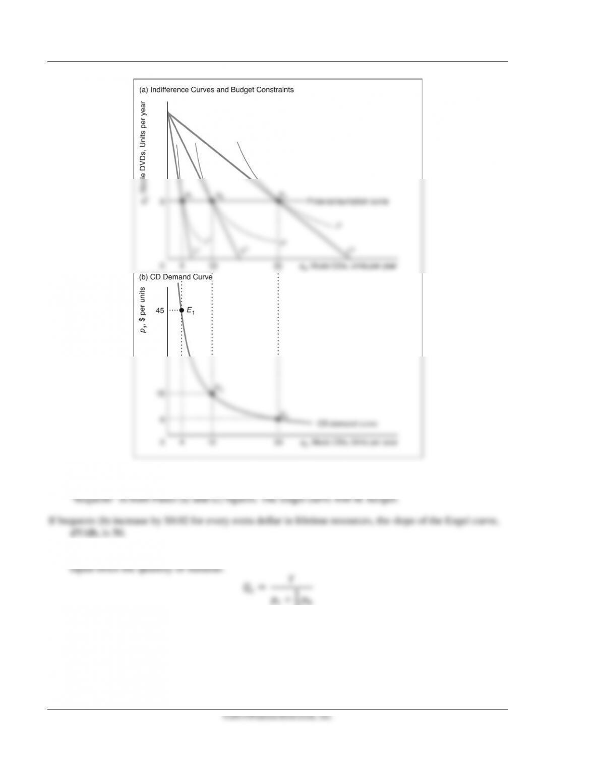
1.7 The figure shows that the price-consumption curve is horizontal. The demand for CDs depends only on
income and the own price, q1 = 0.6Y/p1.
68 Perloff • Microeconomics: Theory and Applications with Calculus, Third Edition
©2014 Pearson Education, Inc.
2.1 The figure will be similar to Panel (a) and Panel (c) of Figure 4.3 in the chapter, but relabel the
vertical “wine” axis as “other goods” (or “fun”) in Panel (a) figure and the horizontal “beer” axis as
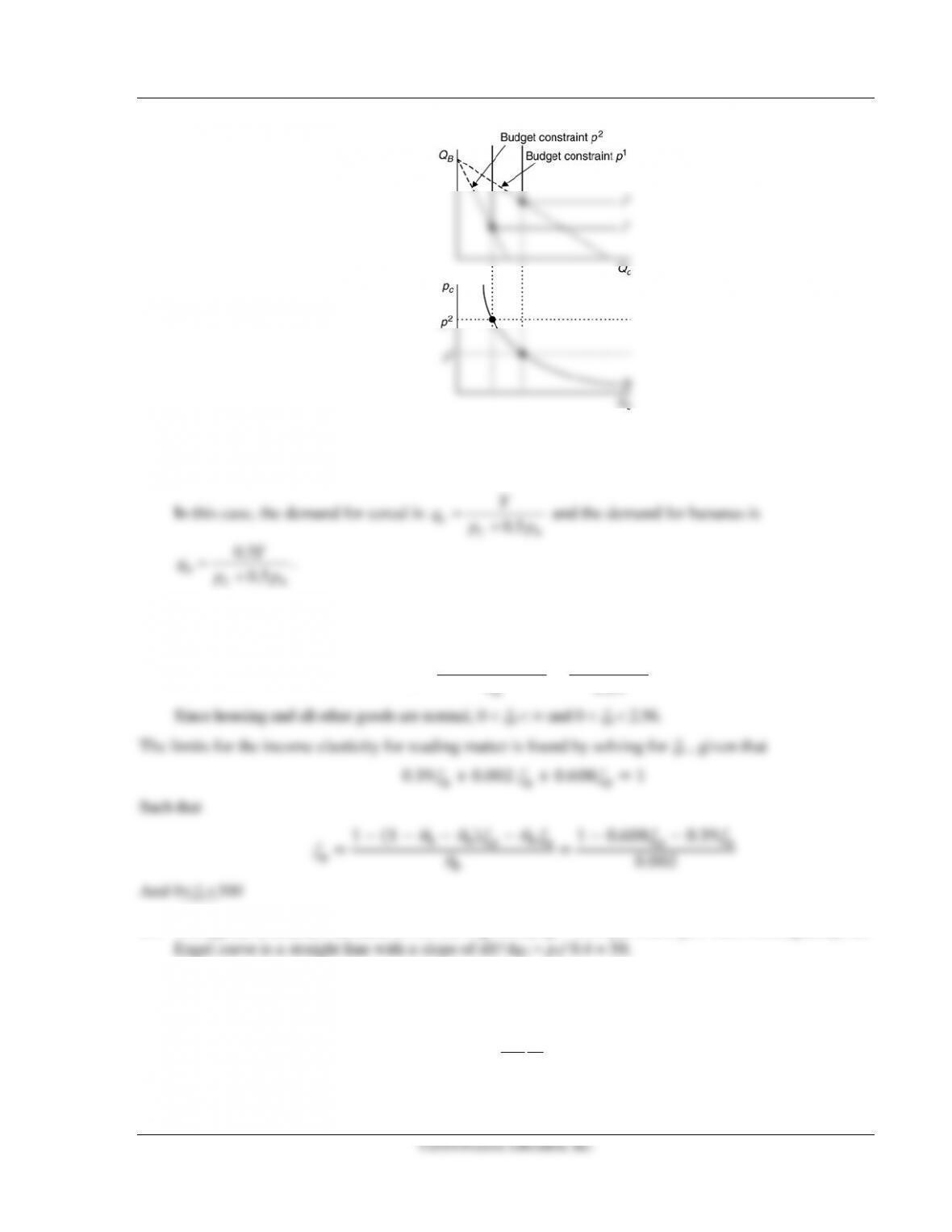
2.2 Guerdon consumes cereal with bananas at a price of pc + 0.5 pb. The quantity of cereal will always
2
Chapter 4 Demand 69
©2014 Pearson Education, Inc.
If Guerdon consumes a bowl of cereal with half a banana, then his utility function is
U = min{qC, 2qB}.
Y
0.5
B
CB
2.3 Using Equation 4.1 from the text where
ξ
h is the income elasticity of housing,
ξ
0 is the income
elasticity of all other goods and
θ
is the budget share of housing and rearranging:
ξ
=1(1
θ
)
ξ
ξ
2.4 The typical consumers demand for DVDs is given by q2 = 0.4Y/p2, where p2 = $20. Consequently, her
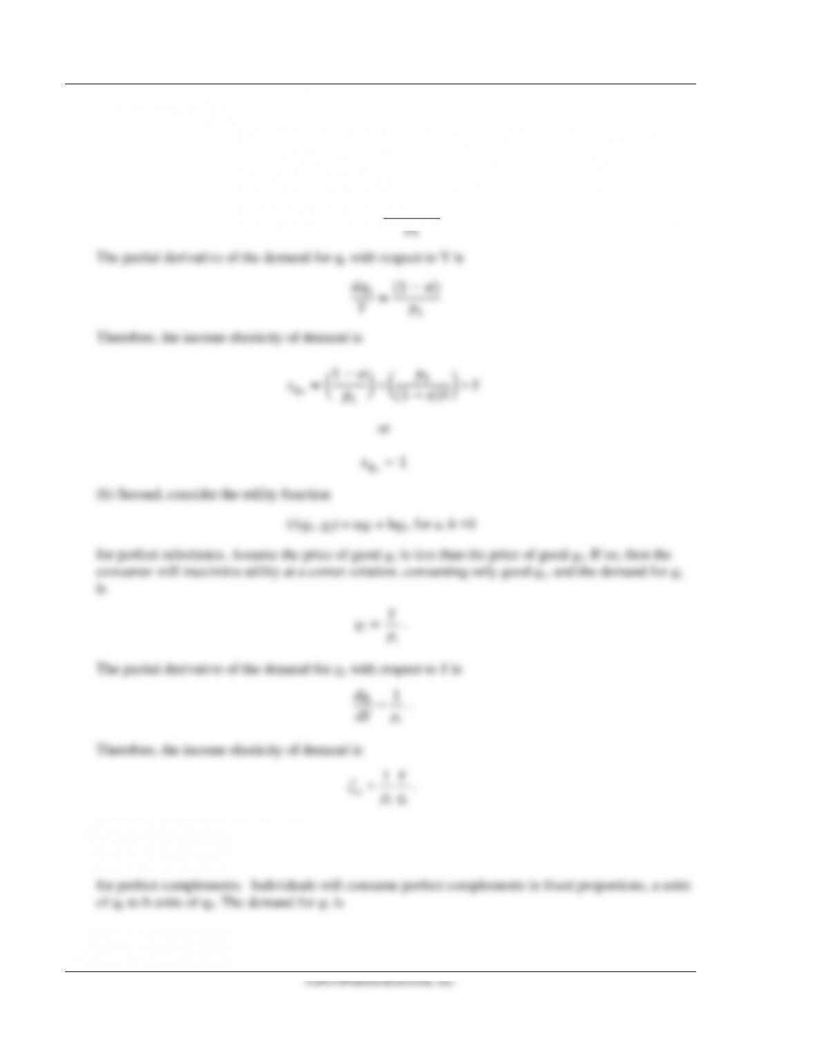
2.5 The income elasticity of demand (or income elasticity) is the percentage change in the quantity
demanded in response to a given percentage change in income, Y:
1
1
q
q
dq Y
dY q
ξ
=
.
70 Perloff • Microeconomics: Theory and Applications with Calculus, Third Edition
(a)First, consider the Cobb-Douglas utility function
U(q1, q2 ) = q1αq2(1–α).
. The demand for q1 is
=(1)
1
11
q
pq
(c) Last, consider the utility function
U(q1, q2) = min{aq1, bq2}, for a, b>0