52 Perloff • Microeconomics: Theory and Applications with Calculus, Third Edition
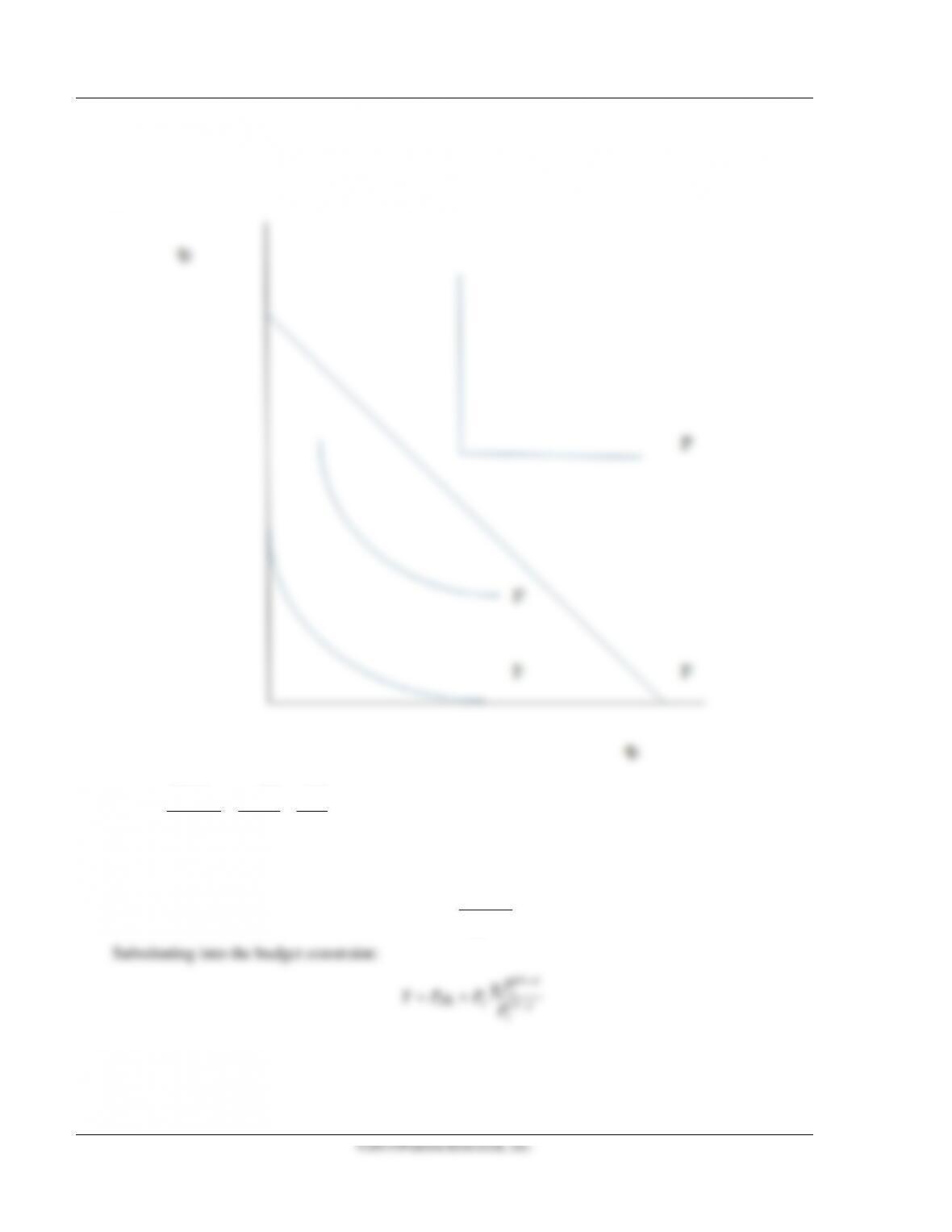
4.7 Perfect complements result in indifference curves shaped like I4 (L–shaped), perfect substitutes in
curves shaped like I3 (straight lines), Cobb-Douglas and Constant-Elasticity–of-Substitution
preferences result in indifference curves shaped like indifference curve I2 (convex), and Quasilinear
preferences like I1 (convex and intersecting the axes).
4.8
11
11 2
11
221
/.
/
Uq q q
MRS Uq q q
ρρ
ρρ
ρ
ρ
−−
−−
∂∂
= = =
∂∂
(Technically, marginal rates of substitution are negative.)
Equating with relative price and solving for q2:
1/1
11
21/1
2
.
qP
qP
ρ
ρ
−
−
=
11 2 1/1
2
ρ
−
Chapter 3 A Consumer’s Constrained Choice 53
©2014 Pearson Education, Inc.
and solving for q1:
11/1
1
12
2
.
Y
qP
PPP
ρ
−
=
+
By symmetry:
21/1
2
21
1
.
Y
qP
PP
P
ρ
−
=
+
4.9
( ) ( )
( ) ( )
( )
( )
11
/.
/1
(1 )
CC FF FF
UC
MRS UF CC
CC FF
αα
αα
αα
α
α
−−
−
−− −
∂∂
= = =
∂∂ − −
−− −
(Technically, marginal rates of
substitution are negative).
Equating MRS with relative price:
( ) ( )
.
1FC
PF F PCC
α
α
−= −
−
4.10 From equation 3.29 and 3.30 in the text:
( )
112
1
,, Y
q PPY P
α
=
and
( )
212
2
, , (1 ) .
Y
q PPY P
α
= −
112
11
γ
212
22
γ
54 Perloff • Microeconomics: Theory and Applications with Calculus, Third Edition
©2014 Pearson Education, Inc.
This is the same result that would occur if all prices and income in the budget constraint were
multiplied by
γ
.
4.11 Diogo’s
2
1
3.
q
MRS q
=
Equating this with the relative price (1/2) and substituting into the budget
constraint, we get
4.12 Consumers spent $932 million in total; $202 million (22 percent) on radios and $730 million (78
12 1 2
4.13 In general, with a Cobb-Douglas utility function of the form
1
12
( )( )Uqq
αα
−
=
4.14 If we plot Good 2on the vertical axis and Good 1 on the horizontal axis, the slope of the indifference
4.15 We can solve this problem by noting that Vasco determines his optimal bundle by equating the ratios
of prices and marginal utilities, such that
=
.
Chapter 3 A Consumer’s Constrained Choice 55
4.16
( )
( ) ( )
2
2 1 2 12 2
22
112 12
q q q qq q
U
qqq qq
+−
∂= =
∂++
( )
( ) ( )
2
1 1 2 12 1
22
212 12
.
q q q qq q
U
qqq qq
+−
∂= =
∂++
( )
21
2
2 12
P PP
+
4.17 The optional value of q1 as a function of a is
=0.5
4.18 The expenditure function is the relationship showing the minimal expenditures necessary to achieve a
specific utility level for a given set of prices.
Kip’s Lagrangian, L, for expenditure minimization is
L=
( )
0.5 0.5
CM
pC p M U C M
λ
+ +−+
,
56 Perloff • Microeconomics: Theory and Applications with Calculus, Third Edition
©2014 Pearson Education, Inc.
2
M
MC
Up
Cpp
=
+
and the optimal value for good M is
2
C
MC
Up
Mpp
=
+
.
Substituting these values for C and M into expenditure function E,
CM
E pC p M= +
.
The expenditure function is
22
((
C
M
CM
CM CM
Up
Up
Ep p
pp pp
= +
++
.
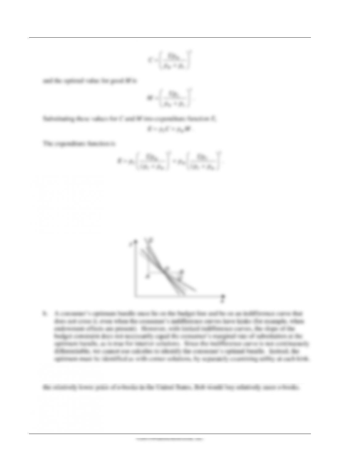
5.1 a. See the figure below. Suppose you are at point O. Assume you are willing to accept AD units of Y
in order to give up OA units of X. On other hand, to buy OB units of X(OA = OB) you are willing
to pay BC units of Y. Therefore you value the same unit of X differently, depending on whether
you want to give it up or you want to buy it. The indifference curve would be DOC and has a
kink at the endowment point. The graph shows different budget constraints at three different
relative prices for X. As you can see, the optimum does not change for small changes of relative
price. Therefore for a range of prices the demand curve for X will be vertical.
6.1 If Bob and Max viewed the two types of books as imperfect substitutes and had the usual convex
indifference curves, they would each buy a mix of e-books and printed books. However, because of
6.2 Describe the indifference curves of the consumer for Canadian and American gasoline: Presumably
the consumer views American gasoline and Canadian gasoline as perfect substitutes, so the
indifference curves are straight lines with a slope of –1.
Chapter 3 A Consumer’s Constrained Choice 57
©2014 Pearson Education, Inc.
Draw the initial budget line where prices are relatively low in the United States, and show the
optimum: For specificity, we assume that, initially, a gasoline budget of Y bought 15 gallons of
gasoline in the United States but only 10 gallons in Canada: budget line L1. The consumer picks the
highest indifference curve, I2, that touches this budget constraint. The optimum, e1, is a corner
solution: The consumer buys gasoline only in the United States. More generally, as long as the budget
line is flatter than the indifference curve, the consumer buys only American gasoline. Letting pa be
the American price and pc be the Canadian price, the slope of the budget line, –pa/pc, is greater
(closer to zero) than the slope of the indifference curves, –1, because pa < pc.
Draw the new budget line where prices are relatively low in Canada and show the new optimum:
After the price change, –pa/pc < –1, so the consumer buys only Canadian gasoline. In the figure, after
the price change, Y buys 15 gallons in Canada and only 10 gallons in the United States: budget line
L1. As a result, the consumer only buys in Canada at e2, where I2 hits L2. Thus, the consumer buys in
whichever country the gasoline is cheapest: a corner solution.
6.3 This explanation is not exactly the same as that in the Challenge Solution because, with the state sales
tax increase, there appears to be some substitution between online purchases and in–store purchases
6.4 If gasoline and ethanol were perfect substitutes, such that 1 gallon of gas equals 1 gallon of ethanol,
then consumers would only purchase the fuel whose price is cheaper. That consumers do not (or that
at least 40 percent of consumers do not behave this way) indicates gas and ethanol are not perfect