Chapter 2 Supply and Demand 33
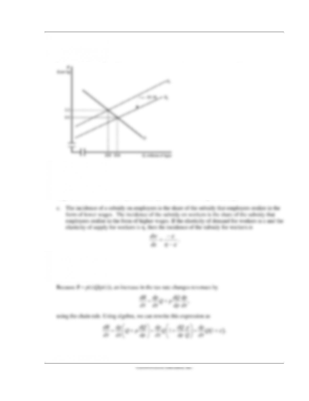
6.6 A subsidy is essentially a negative tax. The supply curve shifts down by the amount of the tax and the
new equilibrium is determined by 286 – 20P = 88 + 40 (p + 1.05). The new equilibrium occurs at a
price of $2.60 and a quantity of 234. Consumers receive $0.70 of the $1.05 subsidy.
6.7 a. A government subsidy paid to employers will shift the labor demand curve up by an amount equal
to the size of the subsidy. The new equilibrium will be at a higher wage with more workers.
b. A reduction in the government subsidy paid to employers will shift the labor demand curve down
by an amount equal to the decrease in the size of the subsidy. The new equilibrium will be at a lower
wage with fewer workers (compared to the equilibrium with the original subsidy).
εη
−
ds
6.8 Differentiating quantity, Q(p(
τ
)), with respect to
τ
, we learn that the change in quantity as the tax
changes is (dQ/dp)(dp/dτ). Multiplying and dividing this expression by p/Q, we find that the change
in quantity as the tax changes is
ε
(Q/p)(dp/d
τ
). Thus the closer
ε
is to zero, the less the quantity falls,
all else the same.
d d dp d dp Q d
ττ τ τ
34 Perloff • Microeconomics: Theory and Applications with Calculus, Third Edition
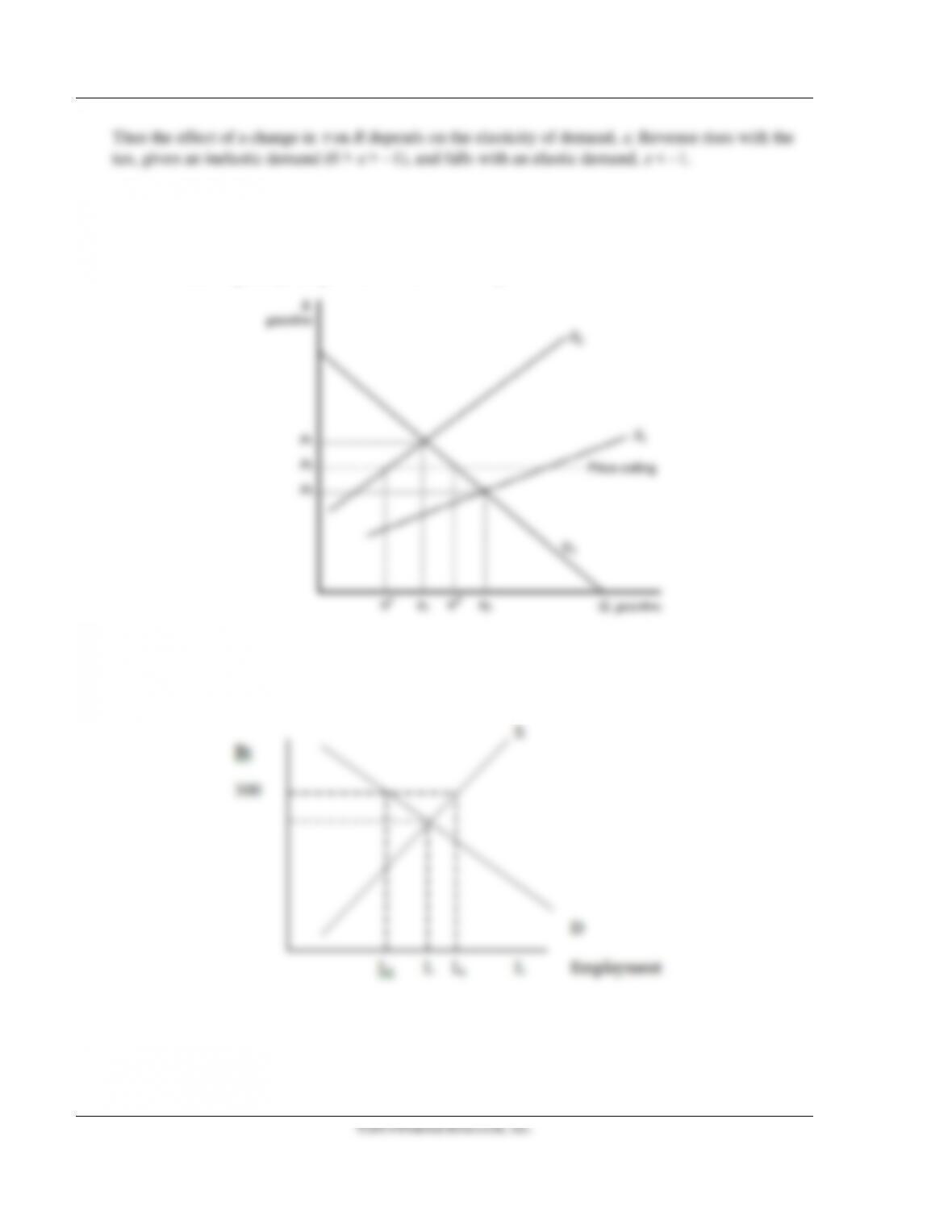
7.1 In the absence of price controls, the leftward shift of the supply curve as a result of Hurricane Katrina
would push market prices up from p0 to p1 and reduce quantity from q0 to q1. At a government imposed
maximum price of p2, consumers would want to purchase qd units but producers would only be willing
to sell qs units. The resulting shortage would impose search costs on consumers making them worse
off. The reduced quantity and price also reduced firms’ profits.
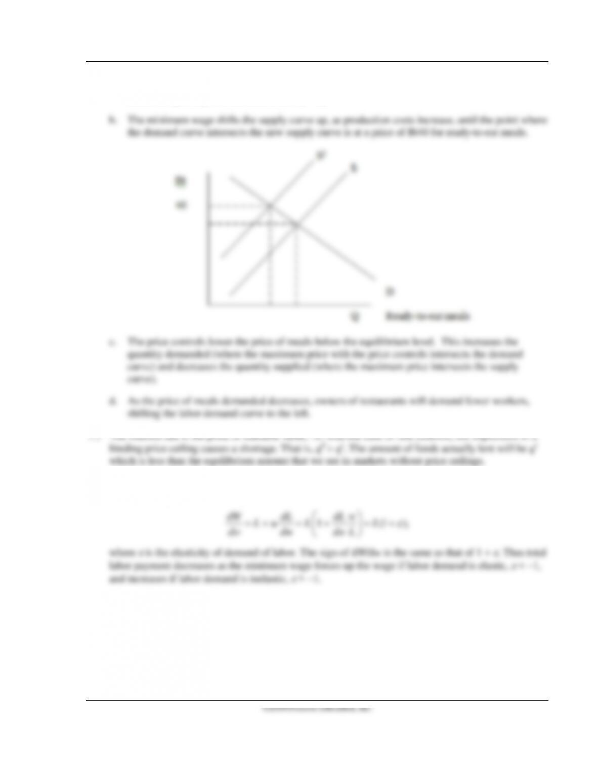
7.2 a. The minimum wage raises the wage above the equilibrium level. This reduces the quantity of
labor demanded (where the Bt300 minimum wage intersects the labor demand curve) and
increases the quantity of labor supplied (where the Bt300 minimum wage intersects the labor
supply curve).
Chapter 2 Supply and Demand 35
Unemployment equals excess labor. That is, unemployment equals the quantity of labor supplied
minus the quantity of labor demanded: Ls – Ld.
7.4 We can determine how the total wage payment, W = wL(w), varies with respect to w by
differentiating. We then use algebra to express this result in terms of an elasticity:
1 (1 ),
dW dL dL w
Lw L L
dw dw dw L
ε
=+=+ =+
where
ε
is the elasticity of demand of labor. The sign of dW/dw is the same as that of 1 +
ε
. Thus total
labor payment decreases as the minimum wage forces up the wage if labor demand is elastic,
ε
< −1,
and increases if labor demand is inelastic,
ε
> −1.
8.1 The supply-and-demand model is useful for making predictions in perfectly competitive markets.
That is, the supply-and-demand model is applicable in markets in which everyone is a price taker,
firms sell identical products, everyone has full information about the price and quantity of goods, and
the costs of trading are low.
36 Perloff • Microeconomics: Theory and Applications with Calculus, Third Edition
©2014 Pearson Education, Inc.
Markets in which the supply-and-demand model has proved useful include agriculture, finance, labor,
construction, services, wholesale, and retail—markets with many firms and consumers and where
firms sell identical products.
a. The market for apples is a competitive, agricultural market.
b. The market with convenience stores is a competitive, retail market.
c. & d. The supply-and-demand model is not appropriate in markets in which there are only one or a
few sellers (such as electricity), firms produce differentiated products (such as music CDs),
consumers know less than sellers about quality or price (such as used cars), or there are high
transaction costs (such as nuclear turbine engines). Electronic games are differentiated products
supplied by three dominant firms.
9.1 If the supply curve were vertical (perfectly inelastic) with a downward-sloping demand curve or if the
demand curve were vertical with an upward-sloping supply curve, then the change in the equilibrium
quantity would not depend on the sizes of the shifts. In the first instance (where the supply curve is
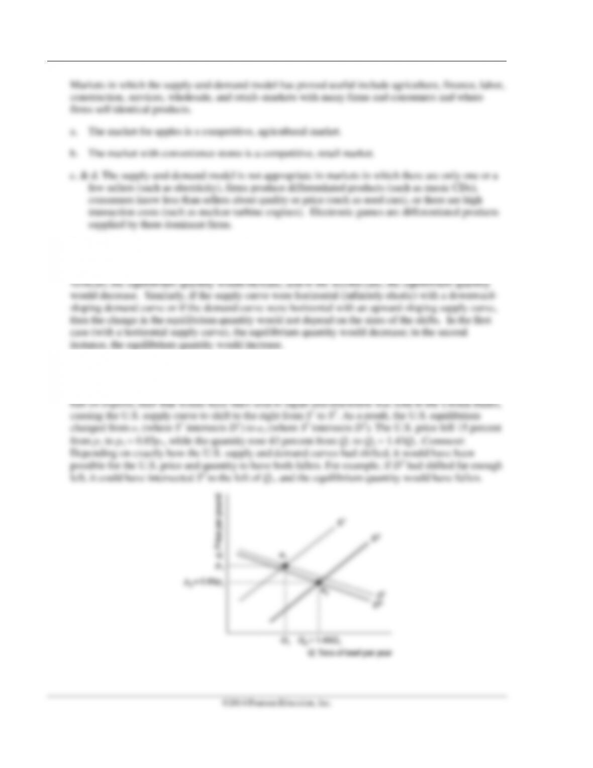
9.2 Shifts of both the U.S. supply and the U.S. demand curves affected the U.S. equilibrium. U.S. beef
consumers’ fear of mad cow disease caused their demand curve in the figure to shift slightly to the
left from D1 to D2. In the short run, total U.S. production was essentially unchanged. Because of the