Chapter 2 Supply and Demand 23
* **
1000 2000
YY Y Y Y
4.6 a. The demand function is Q = 20,000P-0.42, and the inverse supply function is:
1.5
w
PP=
; therefore,
Therefore,
= 16,868.3 (-0.42) P-1.42 = -7084.69P-1.42
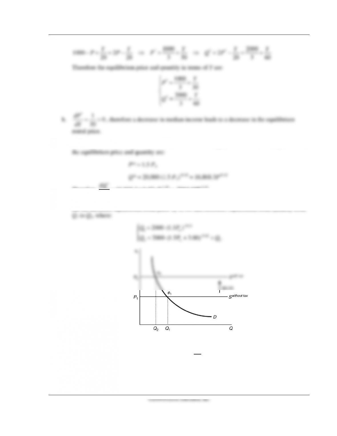
b. As shown in the figure, the total $3.00 specific tax shifts up the supply curve by $3.00. Therefore
0.42
21
2000 (1.5 3.00) .
w
QP Q
−
Math: Suppose the total specific tax is
3.00
τ
=
.
Since equilibrium retail price
1.5
w
PP
τ
= +
, then
10
P
τ
∂= >
∂
, which implies that the specific tax
increases equilibrium retail price.
Since equilibrium retail quantity
0.42
2000 (1.5 )
w
QP
τ
−
=⋅+
, then:
24 Perloff • Microeconomics: Theory and Applications with Calculus, Third Edition
1.42
2000 ( 0.42) (1.5 ) 0,
w
QP
τ
τ
−
∂= ⋅− ⋅ + <
∂
which implies that the specific tax decreases equilibrium retail quantity.
c. With the specific tax in place, the equilibrium price and quantity of cigarettes are:
*
* 0.42
1.5
2000 (1.5 ) .
w
w
PP
QP
τ
τ
−
= +
=⋅+
Then we have:
*1.42 1.42
2000 ( 0.42) 1.5 (1.5 ) 1260 (1.5 ) .
ww
w
QPP
P
ττ
−−
∂=⋅−⋅⋅+=−⋅+
∂
Therefore:
*
1.42
2.42
2.42
() ( 1260 (1.5 ) )
1260 ( 1.42) (1.5 )
1789.2 (1.5 ) .
w
Q
Pw
w
w
P
P
P
τ
ττ
τ
τ
∂−
∂
−
−
∂∂− ⋅ +
=
∂∂
=− ⋅− ⋅ +
= ⋅+
Since the total specific tax is
3.00
τ
=
, then:
*
2.42
()
1789.2 (1.5 3) 0,
w
Q
P
w
P
τ
∂
∂−
∂= ⋅+>
∂
which implies that the change in the wholesale price will have a less negative effect on the
equilibrium quantity if the tax rate increases.
Chapter 2 Supply and Demand 25
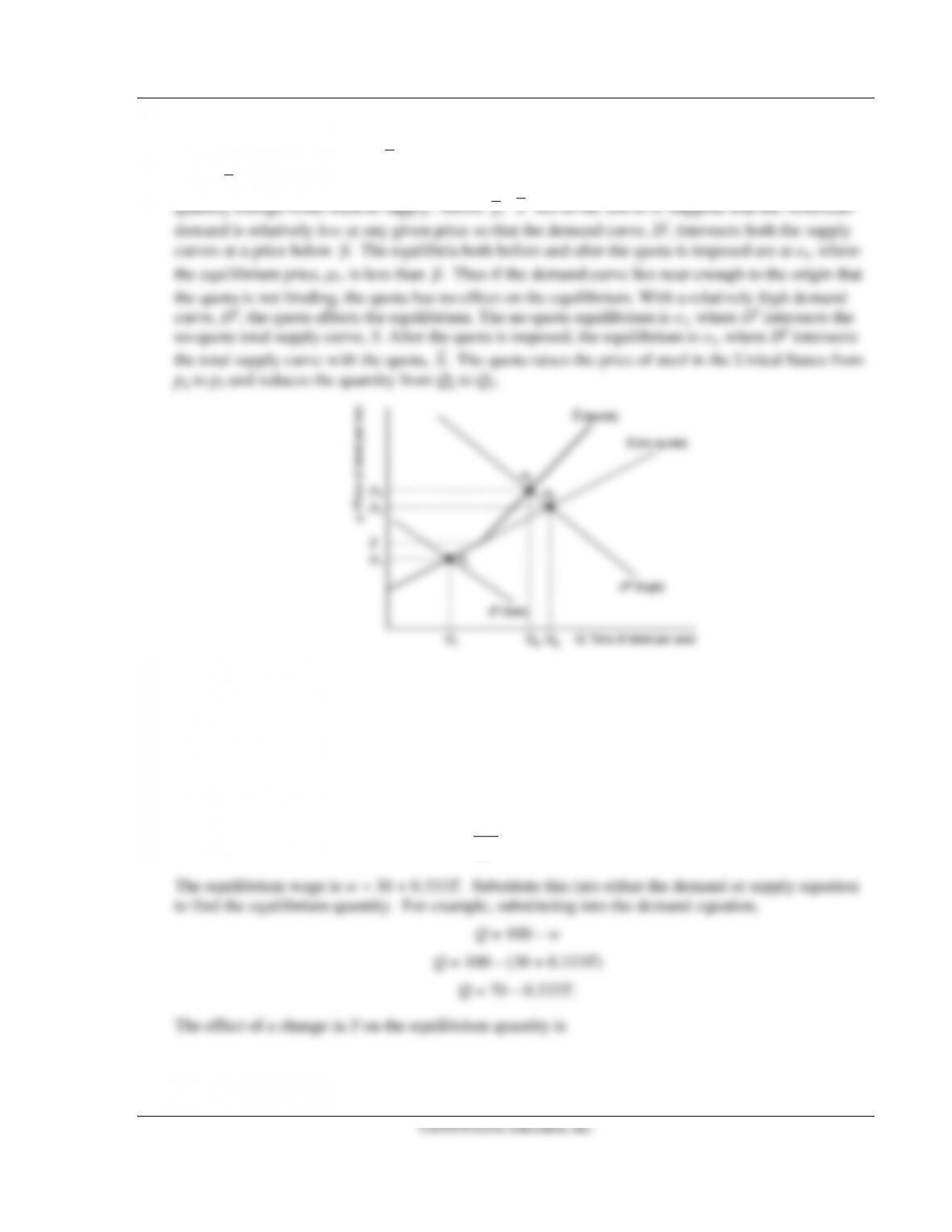
4.7 The figure below reproduces the no-quota total American supply curve of steel, S, and the total
supply curve under the quota,
,S
which we derived in the answer to the previous question. At a price
below
,p
the two supply curves are identical because the quota is not binding: It is greater than the
.p
4.8 The equilibrium wage is that wage where demand equals supply:
100 – w = 10 + 2w – T
90 + T = 3w
w = 30 + 0.333T.
The effect of a change in T on the equilibrium wage is
T
w
∂
∂
= 0.333.
26 Perloff • Microeconomics: Theory and Applications with Calculus, Third Edition
T
Q
∂
∂
= –0.333.
5.1 The demand elasticity is −2.65/21 = −0.13 for prenatal smokers.
5.2 The price elasticity of demand is the percentage change in the quantity demanded, Q, in response to a
given percentage change in price, p, at a particular point on the demand curve:
Q
p
p
Q
∂
∂
=
ε
.
a. Differentiating the first demand curve with respect to p,
2−=
∂
∂
p
Q
.
Substituting this into the elasticity definition with p = 10 and Q = 20,
ε = –2 × (0.5)
ε = –1.
b. Differentiating the second demand curve with respect to p,
5.3 The price elasticity of demand is the percentage change in the quantity demanded, Q, in response to a
given percentage change in price, p, at a particular point on the demand curve:
Q
p
p
Q
∂
∂
=
ε
.
Differentiating the demand curve for small firms with respect to p,
563.1
361.3 −
−=
∂
∂p
p
Qs
.
−
563.0
97.5
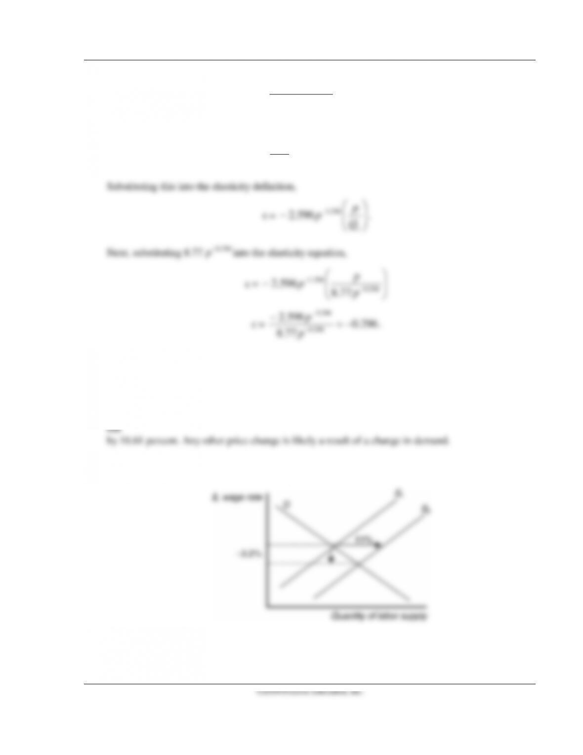
Chapter 2 Supply and Demand 27
ε =
563.0
97.5
361.3
563.0
563.0
−=
−
−
−
p
p
.
Differentiating the demand curve for large firms with respect to p,
296.1
596.2
−
−=
∂
∂p
p
Q
l
.
77.8
296.0
−
p
Since the elasticity of demand for both small firms and large firms is constant along the demand
curves, the elasticity of demand for small firms and the elasticity of demand for large firms is the
same regardless of where they intersect each other.
5.4 The expected percentage price change will be equal to the percentage change in quantity divided by
the price elasticity. 10.4/(−0.626) = −16.61. The increase in supply would cause the price of beef to
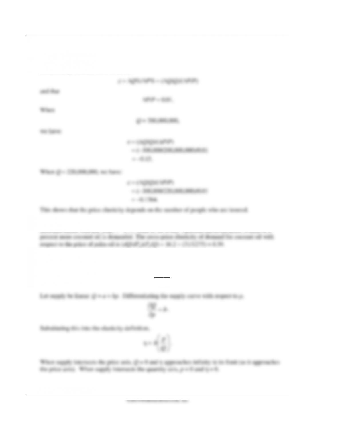
5.5 The numbers suggest that labor demand is inelastic. The supply curve shifts to the right by 11
percent, yet the decrease in equilibrium wage is only 3.2 percent.
5.6 Price elasticity is the percentage change in quantity divided by the percentage change in price.
ε
= −8.3/21 = −0.395. An elasticity coefficient less than 1 indicates an inelastic demand.
28 Perloff • Microeconomics: Theory and Applications with Calculus, Third Edition
5.7 Suppose Q is the number of insured and ∆Q is the change in the number of insured. An increase in
the number of uninsured is the same as a decrease in the number of insured. Therefore an increase in
the number of uninsured by 300,000 can be denoted by ∆Q = −300,000; i.e., number of insured has
decreased by 300,000. Now we know:
5.8 The elasticity of demand is (dQ/dp)(p/Q) = (−9.5 thousand metric tons per year per cent) × (45 cents/1275
5.9 The price elasticity of supply is the percentage change in the quantity supplied, Q, in response to a
given percentage change in price, p, at a particular point on the supply curve:
Q
p
p
Q
∂
∂
=
η
.
Chapter 2 Supply and Demand 29
5.10 The demand curve is Q = 114.8 − 0.0.328p. The supply curve without the ANWR production is
Q = 57.4 + 0.246p. p = 50. The shock will change the supply function to Q = 54.4 + 0.246p.
6.1 Use the following equation to solve for the change in price.
.
dP
d
η
τ ηε
=−
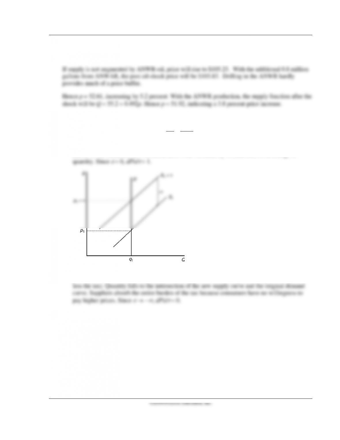
a. If demand is perfectly inelastic, the demand curve is vertical. The supply curve shifts up by $1,
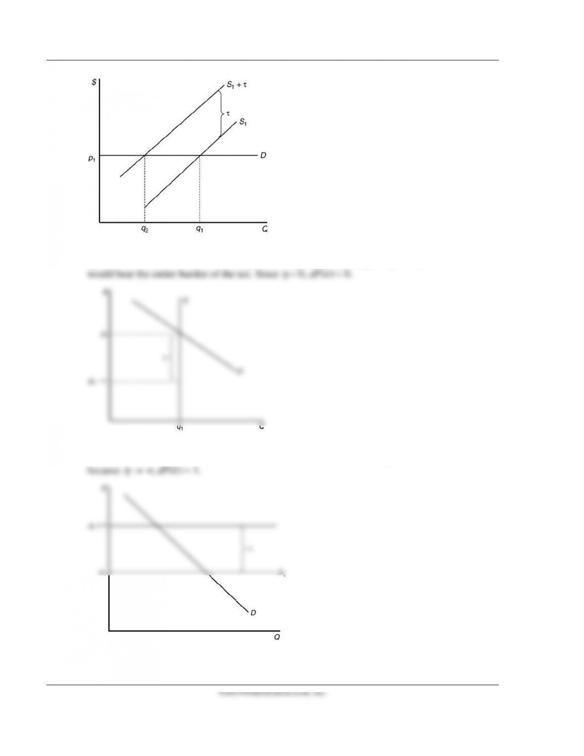
b. The demand curve is horizontal when perfectly elastic. The supply curve shifts up by $1. Price
paid by consumers remains at p (the pre–tax level). Price received by sellers is p –
τ
(the price
30 Perloff • Microeconomics: Theory and Applications with Calculus, Third Edition
c. When supply is perfectly inelastic, the supply curve is vertical. Thus, shifting the supply curve
upward would have no effect on the equilibrium quantity or price paid by consumers. Sellers
d. When supply is perfectly elastic, the supply curve is horizontal. The supply curve shifts up by $1
increasing price by $1. The quantity falls and the incidence falls entirely on the consumer
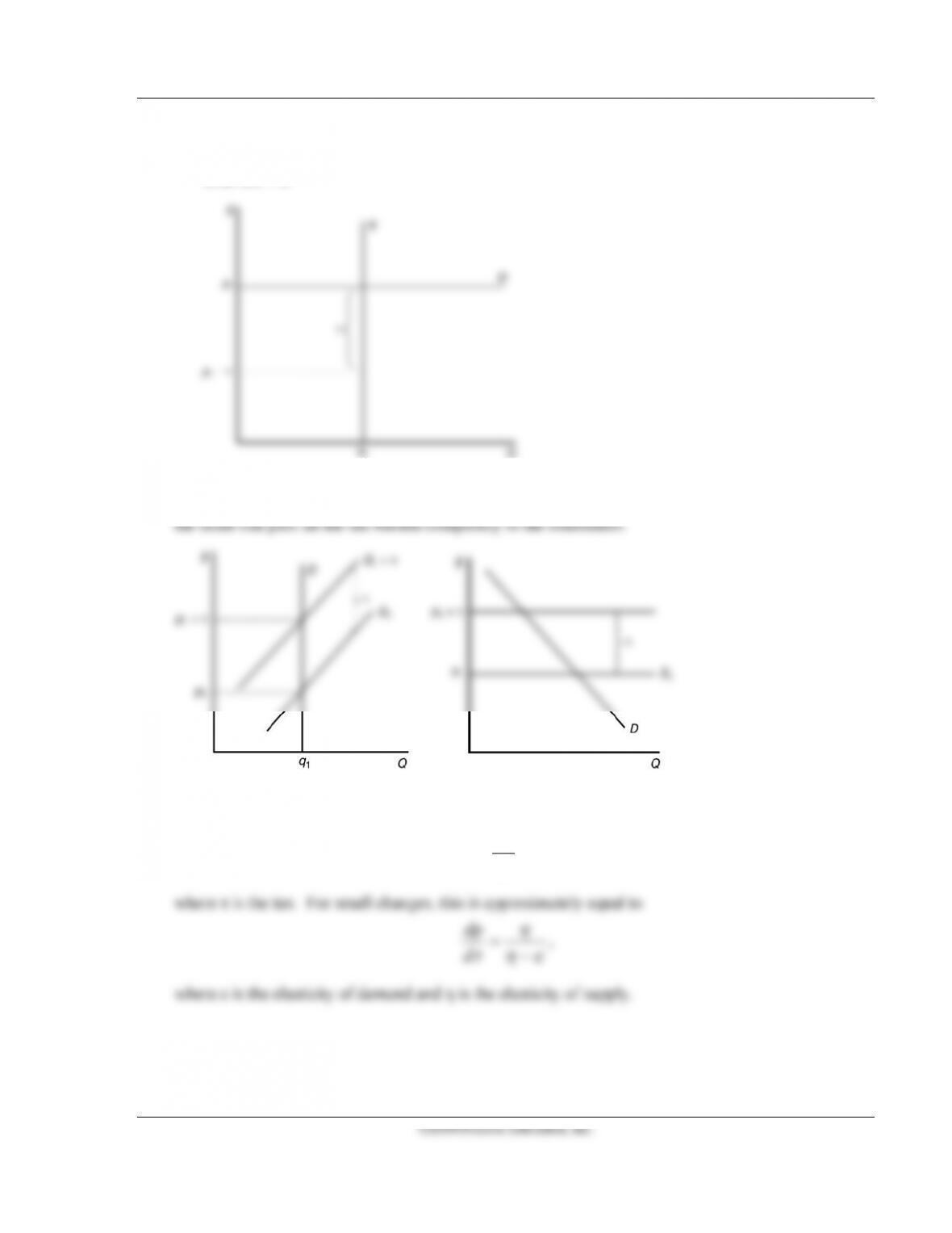
e. If the demand curve is perfectly elastic (horizontal), and the supply curve is perfectly inelastic
Chapter 2 Supply and Demand 31
(vertical), the effect of a tax would be no change in equilibrium quantity and no change in price
paid by consumers, and sellers would bear the entire burden of the tax because
ε
→ −∞ and
η
=
6.2 When the supply curve is upward sloping and the demand curve is vertical (perfectly inelastic demand),
or when the demand is downward sloping and the supply curve is horizontal (perfectly elastic supply)
6.3 The incidence of a tax on consumers is the share of the tax that falls on consumers. The incidence
that falls on consumers is
τ
d
dp
,
32 Perloff • Microeconomics: Theory and Applications with Calculus, Third Edition
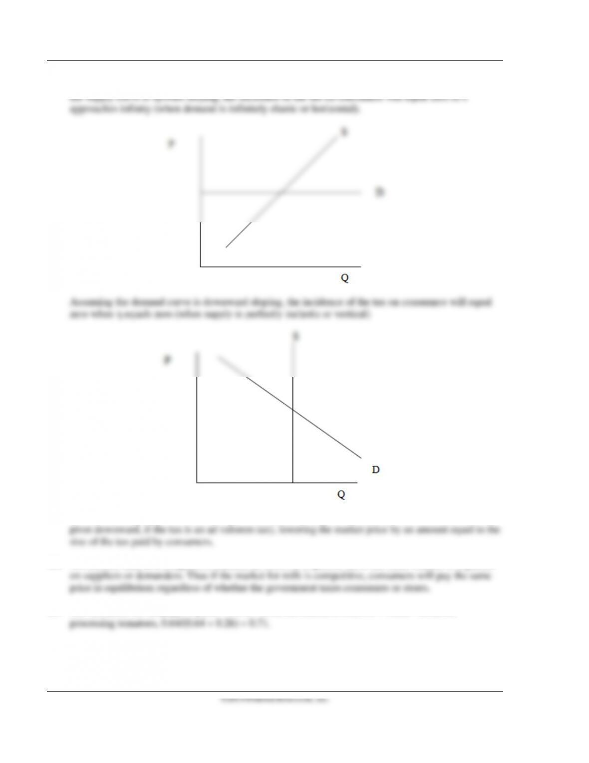
If the pass–through of a tax is 0 percent, then the incidence of the tax on consumers is 0. Assuming
In both cases, a tax on consumers will shift the demand curve downward (or the demand curve will