Chapter 2 Supply and Demand 13
19. Suppose the demand for antibiotics is Q = 100,000. What is the elasticity of demand? If a specific tax
of $1 per dose were levied, who would bear the burden of the tax?
20. Use a graph to show that the incidence of a $1/lb. tax on grapes is the same whether the tax is
shown as a shift in the supply curve (tax on sellers) or the demand curve (tax on buyers). Under
what circumstances would the incidence of the tax be split equally between buyers and sellers?
21. Suppose a tax on beans of $0.05 per can is levied on firms. As a result of the tax, the equilibrium
price increases from $0.20 to $0.22. What fraction of the incidence falls on consumers? On firms?
Suppose the supply elasticity is 0.6. What must the demand elasticity be?
22. If the market demand curve for triple-scoop ice cream cones is QD = 60 − 8p, use the derivative
formula for elasticities to calculate the elasticity of demand when p = $4.
23. Suppose the market supply curve of wagons is QS = −62.5 + 0.5p2. The demand curve is QD = 325 −
2p2. Use Equation 2.27 to determine the incidence of a small tax on consumers.
24. Show that when demand is perfectly elastic, tax incidence is zero.
25. Show that the supply function Q = Ap
ε
has constant elasticity.
Answers to Additional Questions and Problems
1. Possible responses include:
Demand: Price of running shoes (−)
Sock prices (−)
Prices of other sneaker types (+)
Number of people who are regular runners (+)
2. a. The demand curve shifts to the right.
b. The demand curve shifts to the left.
c. The demand curve shifts to the right.
d. The demand curve shifts to the right.
e. The demand curve shifts to the left.
3. a. The supply curve shifts to the right.
b. The supply curve shifts to the left.
c. The supply curve shifts to the left.
d. The supply curve shifts to the left.
e. The supply curve shifts to the left.
14 Perloff • Microeconomics: Theory and Applications with Calculus, Third Edition
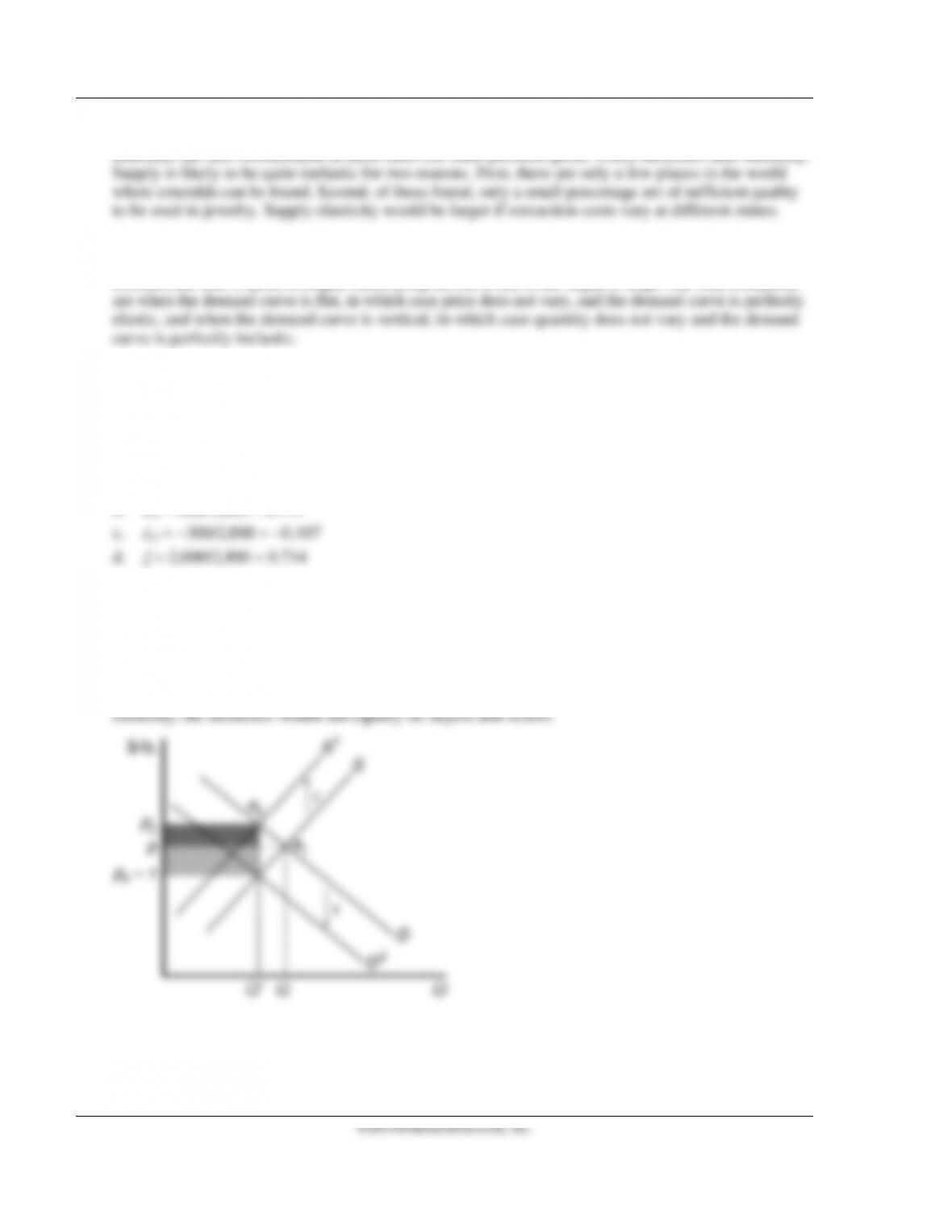
4. Without minimum wages, the equilibrium is
10,000 − 100W = 2,000 + 1,900W
W* = 4
Q* = 9,600.
5. In each case, you must draw a graph that shows the original supply and demand curves, plus the new
curves after the changes. You must then consider whether or not it matters how far the curve shifts in
response to the change in the parameter indicated.
a. Uncertain. In this case, both the supply and the demand curves shift to the right. Quantity will
definitely increase, but whether prices rise, fall, or remain constant depends on the relative sizes
of the supply and demand shifts. In the figure below, because the demand shift is relatively
larger than the shift in supply, prices increase.
Chapter 2 Supply and Demand 15
6. Set QD = QS and solve.
For QS = 20 + p
100 − p = 20 + p
p* = 40
Q* = 60
7. Set QS = QD and solve.
P* = 30
16 Perloff • Microeconomics: Theory and Applications with Calculus, Third Edition
Q* = −10
8. Set QD = QS and solve.
For QD = 300 − 5p
300 − 5p = 60 + 3p
p* = 30
Q* = 150 units.
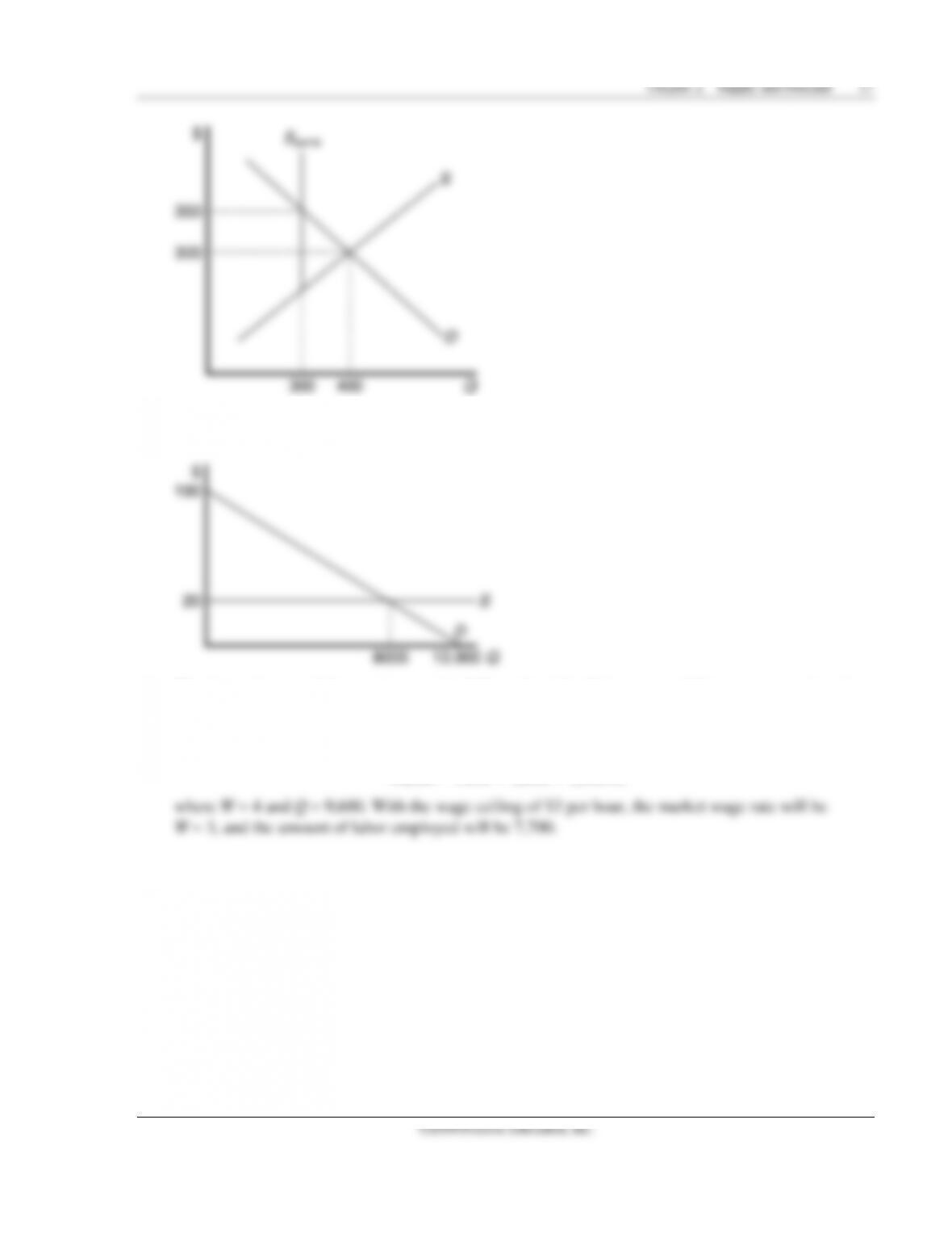
9. The equilibrium solution with no government intervention is
1,000 − 2 p = 100 + p
p* = 300
18 Perloff • Microeconomics: Theory and Applications with Calculus, Third Edition
13. The demand for emeralds is elastic, as they would be categorized as luxury goods rather than necessities.
14. Elasticities that are calculated from linear demand curves are a function of two things. The first is the
slope of the curve, and the second is the ratio p/Q. While the slope of a linear demand curve remains
15.
ε
= (−5/0.25)(1.5/25) = −1.2
16.
ε
= −10(10/100) = −1
17.
η
= (50/0.2)(0.6/50) = 3
18. a.
ε
= −400/(1,000 + 500 − 300 + 2,000 − 400) = −400/2,800 = −0.143
19. Because quantity does not depend on price, demand is perfectly inelastic, and the elasticity is zero.
Consumers would bear the full burden of any specific tax.
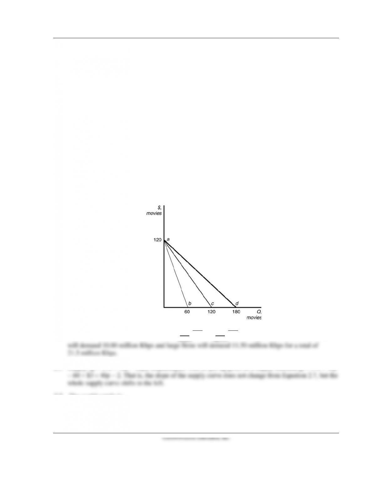
20. In the figure below, the initial equilibrium is at e1. A tax of $1/lb. can be shown by shifting the supply
curve up by $1 (S2) or by shifting the demand curve down by $1(D2). In either case, price paid by
consumers is the same (p2). The upper shaded area is the incidence on consumers; the lower shaded
area is the incidence on suppliers. Using Equation 2.27, if the supply elasticity is equal to the demand
Chapter 2 Supply and Demand 19
21. The incidence on consumers is
ι
= 0.02/0.05 = 0.4. Thus the incidence on firms is 0.6. If the supply
elasticity is 0.6, using formula (2.26), the demand elasticity must be −0.9.
22.
ε
= −32/28 = −1.143.
23. dS/dp = p. dD/dp = −4p. Thus dp/d
τ
= p/[p − (−4p)] = 1/5.
24. The tax incidence is calculated as
η
/(
η
−
ε
). For perfectly elastic demand,
ε
is negative infinity. Hence
the tax incidence is zero.
25. dQ/dp = A
ε
p
ε
− 1. Hence (dQ/dp)(p/Q) = A
ε
p
ε
− 1p/(Ap
ε
) =
ε
, which is a constant.
Answers to Exercises in the Text
1.1 The demand curve for pork is Q = 171 − 20p + 20pb + 3pc + 2Y. As a result, ∂Q/∂Y = 2. A $100
increase in income causes the quantity demanded to increase by 0.2 million kg per year.
1.2 In the figure below, ac is the demand function for college students, and line ab is the demand
function for other town residents. Line ad is the total demand function.
1.3 The total inverse demand function is p =
. +
. . At a price of $0.40, small firms
2.2 The world supply is:
Q = Qa + Qr = (10 + 10p) + (5 + 20p) = 15 + 30p.
20 Perloff • Microeconomics: Theory and Applications with Calculus, Third Edition
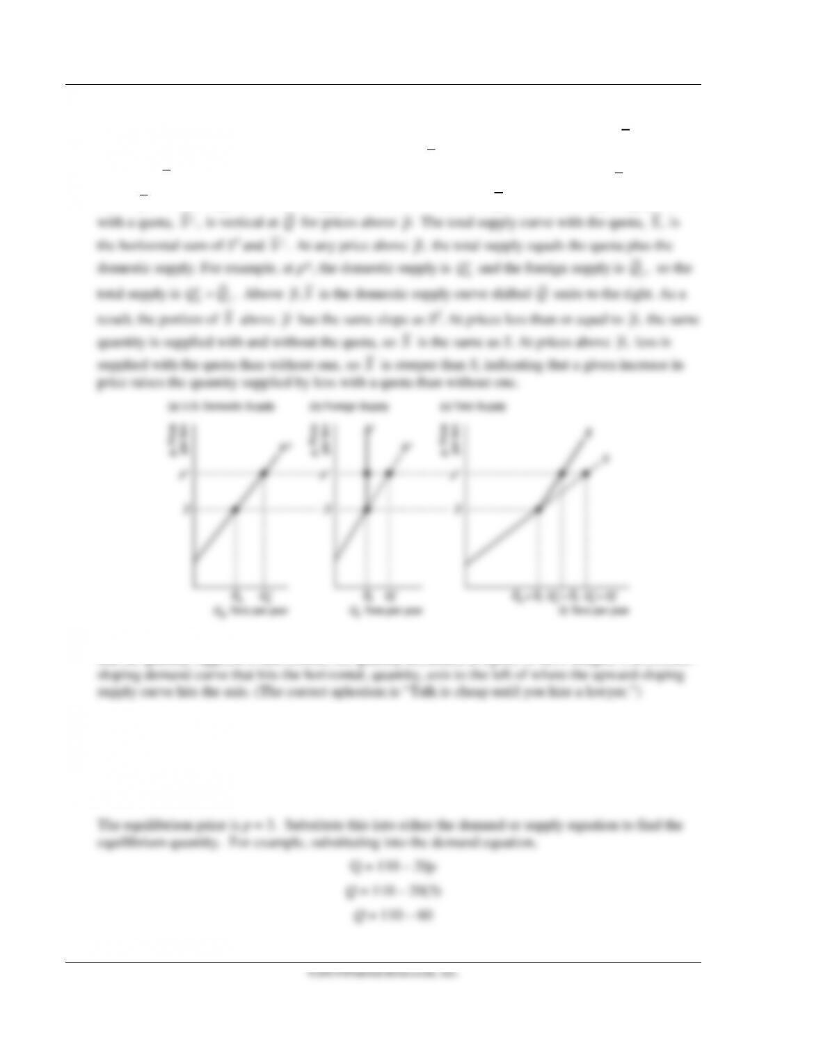
2.3 In the figure below, the no-quota total supply curve, S in panel c, is the horizontal sum of the U.S.
domestic supply curve, Sd, and the no-quota foreign supply curve, Sf. At prices less than
,p
foreign
suppliers want to supply quantities less than the quota,
.Q
As a result, the foreign supply curve under
the quota,
,
f
S
is the same as the no-quota foreign supply curve, Sf, for prices less than
.p
At prices
above
,p
foreign suppliers want to supply more but are limited to
.Q
Thus the foreign supply curve
,p
f
3.1 The statement “Talk is cheap because supply exceeds demand” makes sense if we interpret it to mean
3.2 The equilibrium price is that price where demand equals supply:
110 – 20p = 20 + 10p
90 = 30p
p = 3.
Chapter 2 Supply and Demand 21
Q = 50 units.
3.3 Equating the right sides of the supply and demand functions and using algebra, we find:
0.75 ln(p) = 2.4 + 0.15 ln(pt)
ln(p) = 3.2 + 0.2 ln(pt).
We then set pt = 110, solve for ln(p)
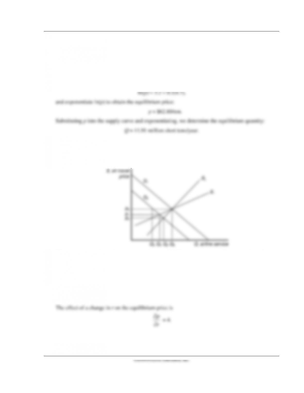
4.1 The demand curve shifts to the left from D1 to D2 by 30 percent, which is the distance between Q0
and Q4. For supply curve S1, the price drops from p0 to p1, a change less than 30 percent. For a steeper
supply curve S2, the price decreases to p2, a larger decrease, yet still smaller than 30 percent.
Accordingly, the equilibrium quantity changes less than 30 percent as well.
4.2 The increased use of corn for producing ethanol will shift the demand curve for corn to the right.
This increases the price of corn overall, reducing the consumption of corn as food.
4.3 The equilibrium price is that price where demand equals supply:
220 – 2p = 20 + 3p – 20r
200 + 20r = 5p
p = 40 + 4r.
r
∂
22 Perloff • Microeconomics: Theory and Applications with Calculus, Third Edition
r
∂
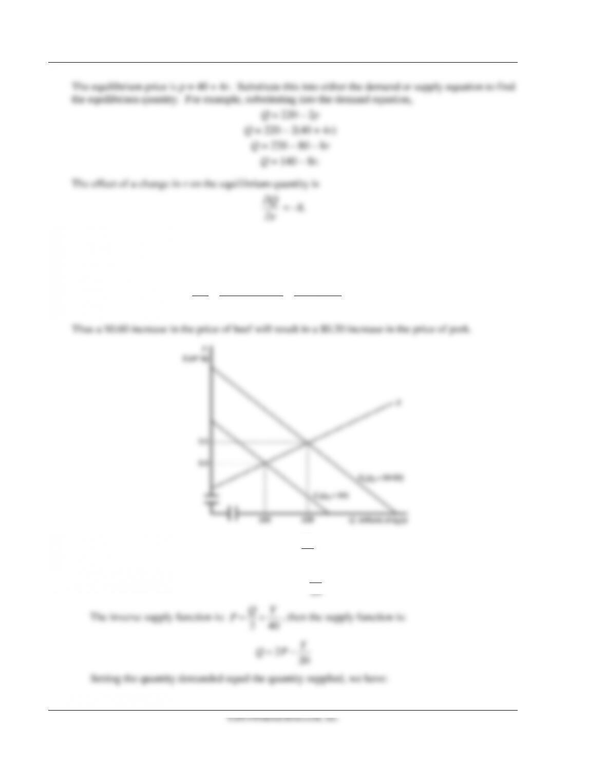
4.4 Start by using equation 2.2 in the text with the usual values for income and chicken prices for demand
206 20 20 b
Q pp=−+
and equation 2.7
88 40Qp= +
for supply. As in solved problem 2.1,
the effect of a change in the price of beef on the price of pork can be shown to be
/20 0.33.
/ / 40 ( 20)
b
b
Dp
p
p Sp Dp
∂∂
∂= = =
∂ ∂ ∂ −∂ ∂ − −
4.5 a. The inverse demand function is:
1000 20
Y
PQ= −+
, then the demand function is:
1000 20
Y
QP
= −+
QY