
317
©2014 Pearson Education, Inc.
Chapter 16
Uncertainty
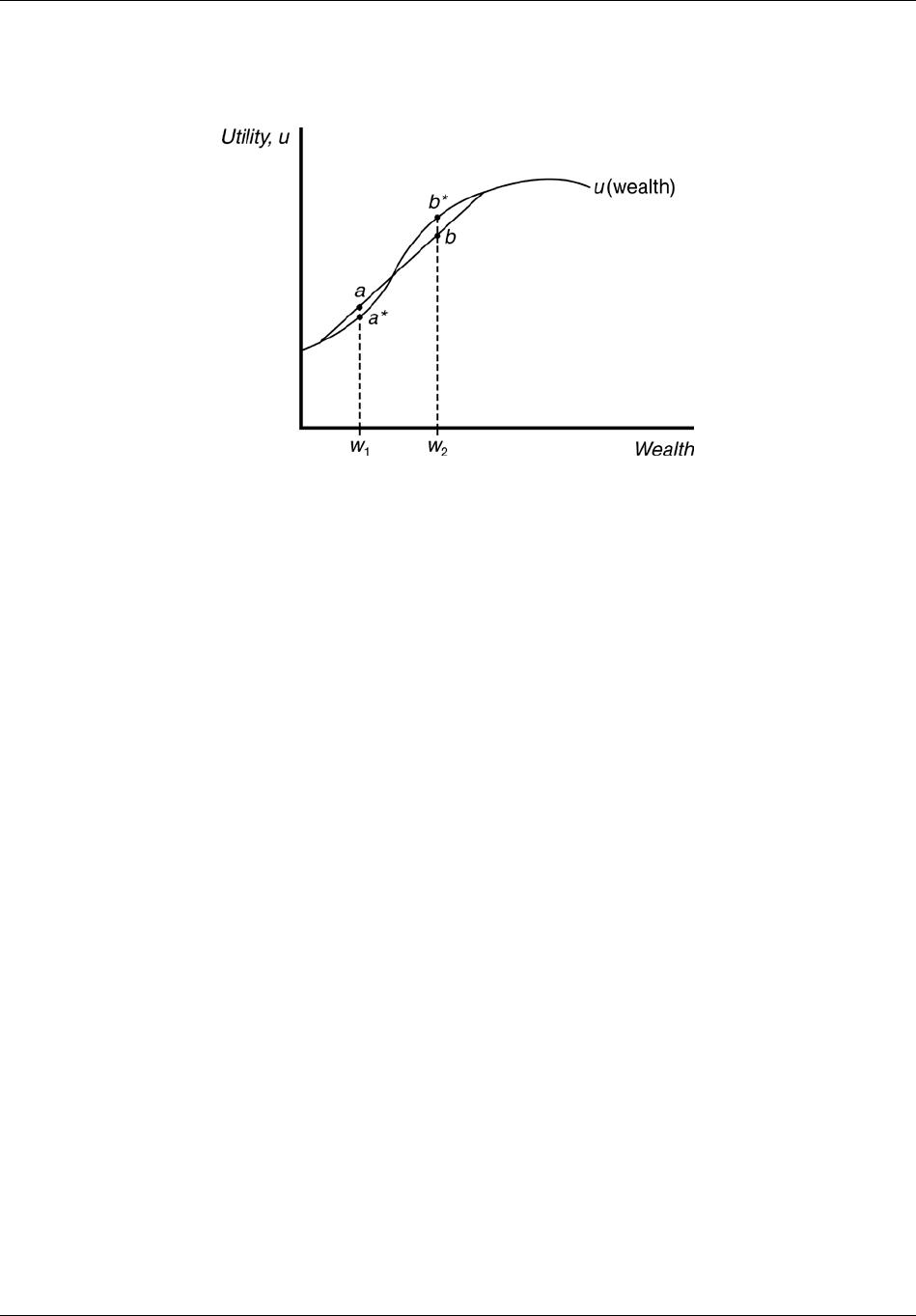
Chapter Outline
16.1 Assessing Risk
Probability
Frequency
Subjective Probability
Probability Distribution
Expected Value
Solved Problem 16.1
Variance and Standard Deviation
16.2 Attitudes Toward Risk
Expected Utility Theory
Risk Aversion
Unwillingness to Take a Fair Bet
Solved Problem 16.2
The Risk Premium
Solved Problem 16.3
Risk Neutrality
Risk Preference
Application: Gambling
Degree of Risk Aversion
Arrow–Pratt Measure of Risk Aversion
Arrow–Pratt Measure and the Willingness to Gamble
Solved Problem 16.4
16.3 Reducing Risk
Just Say No
Application: Harry Potter’s Magic
Obtaining Information
Application: Weathering Bad Sales
Diversification
Application: Employee’s Failure to Diversify

318 Perloff • Microeconomics: Theory and Applications with Calculus, Third Edition
©2014 Pearson Education, Inc.
Insurance
Determining the Amount of Insurance to Buy
Solved Problem 16.5
Fairness and Insurance
Insurance Only for Diversifiable Risks
Application: Limited Insurance for Natural Disasters
16.4 Investing Under Uncertainty
How Investing Depends on Attitudes Toward Risk
Risk–Neutral Investing
Risk–Averse Investing
Investing with Uncertainty and Discounting
Solved Problem 16.6
16.5 Behavioral Economics and Uncertainty
Biased Assessment of Probabilities
Gambler’s Fallacy
Overconfidence
Application: Biased Estimates
Violations of Expected Utility Theory
Framing
Certainty Effect
Prospect Theory
Comparing Expected Utility and Prospect Theories
Properties of Prospect Theory
Teaching Tips
Chapter 16 begins with a review of some basic statistics. If the class you are teaching has a statistics
prerequisite, you may be able to either skip this review all together or give it a brief treatment to refresh
the students’ memories. The von Nuemann–Morgenstern utility material can be included as part of utility
analysis (Chapter 4) if you will not have time to cover this chapter separately.
When describing attitudes toward risk, beware of the classroom demonstration. I once watched a
professor come pretty close to losing $10 on a coin flip bet in an effort to demonstrate risk neutrality.
When circumstances are artificial, such as classroom experiments, or there is value to posturing by
participants, risk–preferring behavior is much more likely than in a true empirical test. (However, I also
know two professors who were able to “win” a lot of hours of community service from students in a
demonstration that showed quite clearly that the students were overconfident in their betting and did
not fully understand the odds of winning casino-style games.)
One interesting application of this material is the complication caused by scope economies in regulated
industries. In regulated industries, one way to determine a fair rate of return is to compare the rates of
return to nonregulated industries in a similar risk class. Under such a system, a regulated telecommunications
provider’s allowable earnings would end up being determined in part by the level of risk that regulators
believe they are exposed to. Although the portfolio effect of multiple output production can be used to
create a reduction in risk by evening out revenue flows, there is also a risk-concentrating effect of using
the same capital to produce multiple outputs. For example, in 1988, in Hinsdale, Illinois, a fire at a

Chapter 16 Uncertainty 319
©2014 Pearson Education, Inc.
telecommunications switch caused the complete loss of service to all outputs provided by that switch.
WATS lines, 800 service, residential, and business calling were all interrupted. While the switch is in
operation, the telephone company receives the benefits of reduced production cost (scope economies),
as well as a reduction in revenue fluctuations through diversification. However, producing all of these
outputs using the same switch concentrates risk. If one type of risk is accounted for, but the other is not,
the firm may be misclassified.
You can also discuss risk in the context of commodities that your students purchase. For those who travel
to Jamaica or other island spring break destinations, ask how much they would be willing to pay for trip
insurance. Then turn the tables and ask under what circumstances an insurer would be willing to provide
such insurance and at what price relative to trip cost.
The final section on behavioral economics is filled with opportunities for classroom applications and
examples because students are aware of so many real–life applications relating to seemingly inconsistent or
irrational behavior. This might also be an opportunity for a macroeconomics tie-in to risk–taking by banks
and mortgage lenders during the recent financial crisis.
Additional Applications
How Farmers Reduce Risk1
Farmers face both financial and production (low yield per acre) risks. Financial risks include changes in
output price, physical factor input cost, and labor cost. Production risks are due to weather such as droughts,
and freezes, pests, diseases, and floods. A survey of California farmers showed that they take direct
actions, diversify, buy insurance, and hedge to reduce risks.
Direct approaches to reducing yield variability include installing wind machines, helicopters, and other
equipment to protect crops during sudden frosts, and installing irrigation systems to protect against droughts.
One–fifth of California farmers gain some risk protection from using government programs that stabilize
prices (see Chapter 9). A few (1.2 percent) sign labor contracts to reduce wage fluctuations.
Nearly a quarter, 23.4 percent, of California farmers forward contract. A forward contract is signed before
the growing season and usually specifies a price (or range of possible prices) to be paid upon delivery. If
the contract guarantees the farmer a price of $5 per bushel, the gains or losses of higher or lower prices are
borne by the buyer. Any farmer can forward contract if some other party is willing to absorb the risk.
Only 6.2 percent of farmers hedge to reduce risks. Many farmers fail to hedge because no futures or
options market exists for their crops, they do not understand hedging, or they do not trust these markets.
These farmers favor forward contracts because they can lock in prices for longer periods of time.
Crop insurance, which protects the farmer against unexpected drops in yield, is used by 24.4 percent of
California farmers. Crop insurance is only available for some crops. Because federal crop insurance
programs were designed primarily for farmers in the Midwest, they are not always attractive to California
farmers. A farmer can collect only if the loss exceeds a certain percentage of the average yield. Because
California farmers face less yield variability and are less likely to collect on the insurance, the federal rates
are often not attractive for many of them. Only 60 percent of the farmers who do buy crop insurance buy it
every year. About one-third buy it only in years where they expect adverse weather conditions. If they
have better information than federal insurers, this practice can lead to adverse selection.
1Based on Steven C. Blank and Jeffrey McDonald, “How California Agricultural Producers Manage Risk,” California
Agriculture, 49(2), March-April 1995:9–12, and Venner and Blank (1995).

320 Perloff • Microeconomics: Theory and Applications with Calculus, Third Edition
©2014 Pearson Education, Inc.
California farmers’ main approach to avoiding financial and yield risks is to diversify across crops or
between agricultural and nonagricultural activities. Nearly half of the farmers diversify across agricultural
activities. Nearly two–thirds (63 percent) of producers receive nonagricultural income, accounting for 47
percent of their total family income. Diversification helps protect against both financial and production
risks.
1. How has the globalization of agricultural markets affected U.S. farmers’ need for insurance?
2. Suppose a new weather forecasting method was derived that was 50 percent more accurate than the
current method. How would this affect the insurance market?
3. What is the relationship between risk and length of product cycle?
Discussion Questions
1. How can you determine how risk averse someone is?
2. Do you know someone who is strictly risk preferring? What evidence do you have?
3. I’m convinced that one of my colleagues would try to drive home blindfolded if offered a large
enough bet. Why would he do that? What must be his attitude toward risk?
4. Should governments prohibit gambling? Should governments run legalized gambling lotteries?
5. Winnings from gambling (whether legal or not) are subject to U.S. income tax. You may, however,
deduct your losses up to the extent of your winnings. How do these tax laws affect an individual’s
willingness to gamble or the size of the gamble?
6. Are both the standard deviation and beta measures of risk?
7. Some states forbid insurance rate discrimination on the basis of gender. Without such laws, insurance
companies would charge young male drivers higher rates because they are more likely to be involved
in accidents. Discuss the efficiency and equity implications of such antidiscrimination laws.
8. Why would a company offer a “money-back guarantee if not completely satisfied” if the firm knows
that it is impossible to satisfy all consumers completely?
Additional Questions and Problems
1. Suppose you are selling kites on the boardwalk at the New Jersey shore as your summer job. Every
fourth person that passes you selects a kite at random and buys it. One–half of your kites sell for $8,
and the other half sell for $4. If 100 people per hour pass by, what is your expected revenue for six
hours work?
2. In Problem 1, of the people who bought kites, what are the variance and standard deviation of
revenue per person?
3. Many states run lotteries of various kinds. One of the most popular is a daily number game where
an individual buys a $1 ticket with a number of their choosing between 000 and 999. The payoff is
typically $500. Would a strictly risk-neutral person buy such a ticket? What payoff would ensure
that at least some people who are risk averse would buy a ticket?

Chapter 16 Uncertainty 321
©2014 Pearson Education, Inc.
4. Draw a utility function such that the person is risk preferring with respect to a small gamble, but risk
averse with respect to a large gamble.
5. What would be the price of fair insurance for a $20,000 motor home for one year, assuming that
during that year there is a 0.02 percent chance that it will be destroyed in an accident, leaving a
$3,000 salvage value and no chance of any partial loss? Assume that the owner keeps the salvage
value.
6. Suppose it costs a corporation an additional $500 in transactions costs to have two executives fly
separately rather than together. If they were both killed, they would lose $5 million in profits. Given
that a probability of any single flight crashing of 0.000000432, should a risk-neutral firm separate the
executives?
7. Why do most investment counselors typically recommend that their clients alter their portfolio of
stocks and bonds as they age?
8. Would you want to purchase auto insurance from a company that claims to turn down no one and
charges all drivers the same price?
9. Why don’t employers spend whatever is required to eliminate all risks from jobs (such as
construction work)? Would employees want the employer to do so?
10. Twenty years ago, almost no one wore helmets while skiing. Now many skiers wear them. What
could have caused such a change?
11. Using information from the utility function in the figure (in the Application: Gambling) on page 574
of the text, what would be Sylvia’s preference between the following two games: (i) receiving W3
with certainty; (ii) receiving W1 or W5 with equal probabilities?
12. In Figure 16.4 of the text, what is the optimal choice of the risk-averse owner if the probability of
high demand and low demand is 90 percent and 10 percent, respectively?
Answers to Additional Questions and Problems
1. Expected revenue would be the product of expected sales (1,003.25) and expected price
(0.53 $4 + 0.53 $8), or $150.
2. The variance is 0.5(8 – 6)2 + 0.5(4 – 6)2 = 4. The standard deviation is $2.
3. A person who is strictly risk neutral would not buy a ticket because the expected value of the ticket
is only 50 cents (0.0013500). The payoff would have to be at least $1,001 to ensure that some risk-
averse individuals would play. This, however, would result in losses for the lottery since, on average,
they would pay out more than they took in.
322 Perloff • Microeconomics: Theory and Applications with Calculus, Third Edition
©2014 Pearson Education, Inc.
4. Such a utility function would be opposite of the Friedman-Savage Utility function. The expected
utility of a small gamble (a) is greater than if the outcome were certain (a*), while the expected utility
of a large gamble (b) is less than if the outcome were certain (b*).
5. The expected value of the motor home is $19,660 = (0.02 × $3,000 + 0.98 × $20,000). Thus fair
insurance for the motor home would cost $340 = (0.02 × $17,000), where $17,000 is the net loss from an
accident.
6. They should fly together, as the expected loss in profits due to a possible crash is only about $2.
7. As individuals age, their ability to make up losses due to large swings in financial markets is reduced,
making them more risk averse. Typically, fund managers recommend higher risk (variance), higher
expected return investments for long-term investors, as market fluctuations will be averaged out over
time. For investors near retirement, lower return, lower variance investments are preferred.
8. An adverse selection problem occurs if the insurance company does not turn away bad drivers. Because
prices are set by the insurance company such that the expected payout is less than the sum of all
premiums, good drivers end up subsidizing bad drivers if premiums are uniform. As a good driver,
you would be better off insuring with a firm that turns away drivers with a history of previous accidents.
9. Employers do not remove all risk from work environments for two reasons. First, it may not be
possible to eliminate all risk, no matter what the expenditure. Second, it may be cheaper to pay
employees to accept the risk in the form of a differential rather than abate it. Employees have
different levels of risk aversion. Those employees who are highly risk averse will prefer lower wage,
safe jobs. Less risk–averse workers with a high marginal utility of income will prefer to accept some
risk in exchange for higher pay.
10. There are several possible reasons. The first is that skiing might be more dangerous than it was
20 years ago (an increase in the probability of injury). Second, the risk may be the same, but skiers
may be more aware of the risks (better information). Finally, skiers may be more risk averse than
they were 20 years ago and so are less willing to risk an injury.
11. Sylvia will be indifferent between the two games, as the expected value of the bet is equal to the
payoff with certainty.
12. The expected payoff with 90 percent and 10 percent probability is 40 × 90% + 0 × 10% = 36 > 35.
Hence the owner will choose to invest in this business.