224 Perloff • Microeconomics: Theory and Applications with Calculus, Third Edition
©2014 Pearson Education, Inc.
1.13 This test is relevant because if the club were maximizing revenue, it would be operating at the level
MR = 0, where the elasticity is −1.
2.1 A monopolist may set price equal to marginal cost if other firms can enter costlessly. If there is free
2.2 Amazon’s Lerner Index was (p − MC)/p = (359 – 159)/359 ≈ 0.557. Using Equation 11.11, we know
2.3 The Lerner Index is (84.95 − 37)/84.95 = 0.56. Hence Stamps.com believes that it faces a demand
2.4 Given that Apple’s marginal cost was constant, its average variable cost equaled its marginal cost,
$200. Its average fixed cost was its fixed cost divided by the quantity produced, 736/Q. Thus, its
average cost was AC = 200 + 736/Q. Because the inverse demand function was p = 600 − 25Q,
Apple’s revenue function was R = 600Q − 25Q2, so MR = dR/dQ = 600 − 50Q. Apple maximized its
2
2.5 The price/marginal cost ratio is 99/45.37 = 2.18. Lerner Index is
/ 99 45.37/99 0.542.−=− =P MC P
2.6 a. Setting MR = MC we get 1.98 − 2 × 0.00198Q = 0. Solving the equation we get Q* = 500.
2.7 a. Assume demand is
1
D
. Then, the consumer surplus is
++,adh
the producer surplus is b + i,
and social deadweight loss is c + e. If the monopoly behaves like a price taker, the quantity will
Chapter 11 Monopoly and Monopsony 225
c. Under the convex demand curve,
3
,D
the price and quantity will be the same as in the linear
case. But under the price–taker assumption, the quantity supplied will be Q3. Consumer surplus
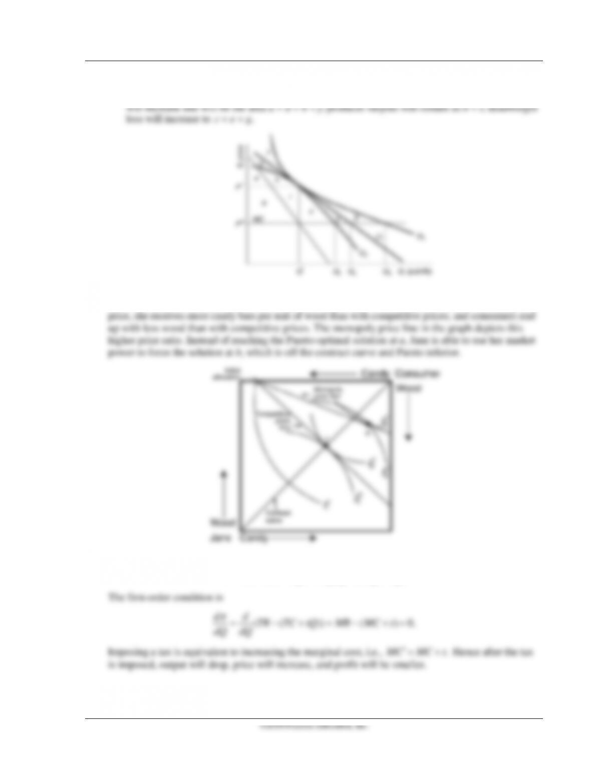
2.8 To be on the contract curve (Pareto efficiency) requires that all goods be traded at competitive prices.
Because Jane is a monopolist, she sets the price of wood above the competitive price. At this higher
3.1 The total profit is total revenue minus total cost and tax.
( ) () (() )
π
=− += − +TR TC tQ P Q Q C Q tQ
226 Perloff • Microeconomics: Theory and Applications with Calculus, Third Edition
3.2 A monopoly will maximize profits by picking a price, p, such that
+
=
ε
1
1
MC
p
.
+
+
=
ε
1
1
1
2
M
p
.
In turn,
+
−
+
+
=−
εε
1
1
1
1
1
12 MM
pp
+
=−
ε
1
1
1
1
2
pp
.
If ε equals –2, then the change in price is
−
+
=−
2
1
1
1
1
2
p
p
=$2.00.
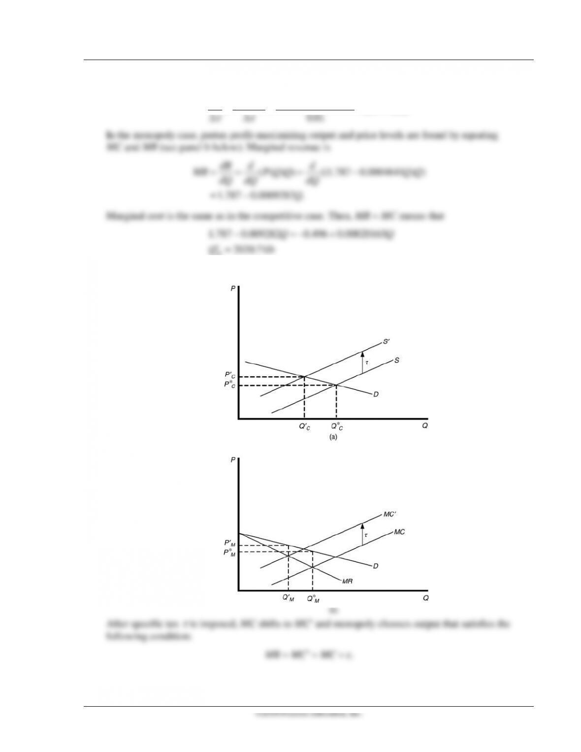
3.3 In the competitive case, equilibrium is found by equating supply and demand curves, D = S:
− =−+1.787 0.0004641 0.496 0.00020165 .QQ
Then
=
=
*
*
3429.2151 lb
0.19550 $/lb.
C
C
Q
P
′=
′=
3414.1945 lb
0.20247 $/lb.
C
C
Q
P
Chapter 11 Monopoly and Monopsony 227
This suggests that tax incidence in the case of competition is
−
∆−
‘*
0.20247 0.19550 0.7 70%.
CC
PP
p
228 Perloff • Microeconomics: Theory and Applications with Calculus, Third Edition
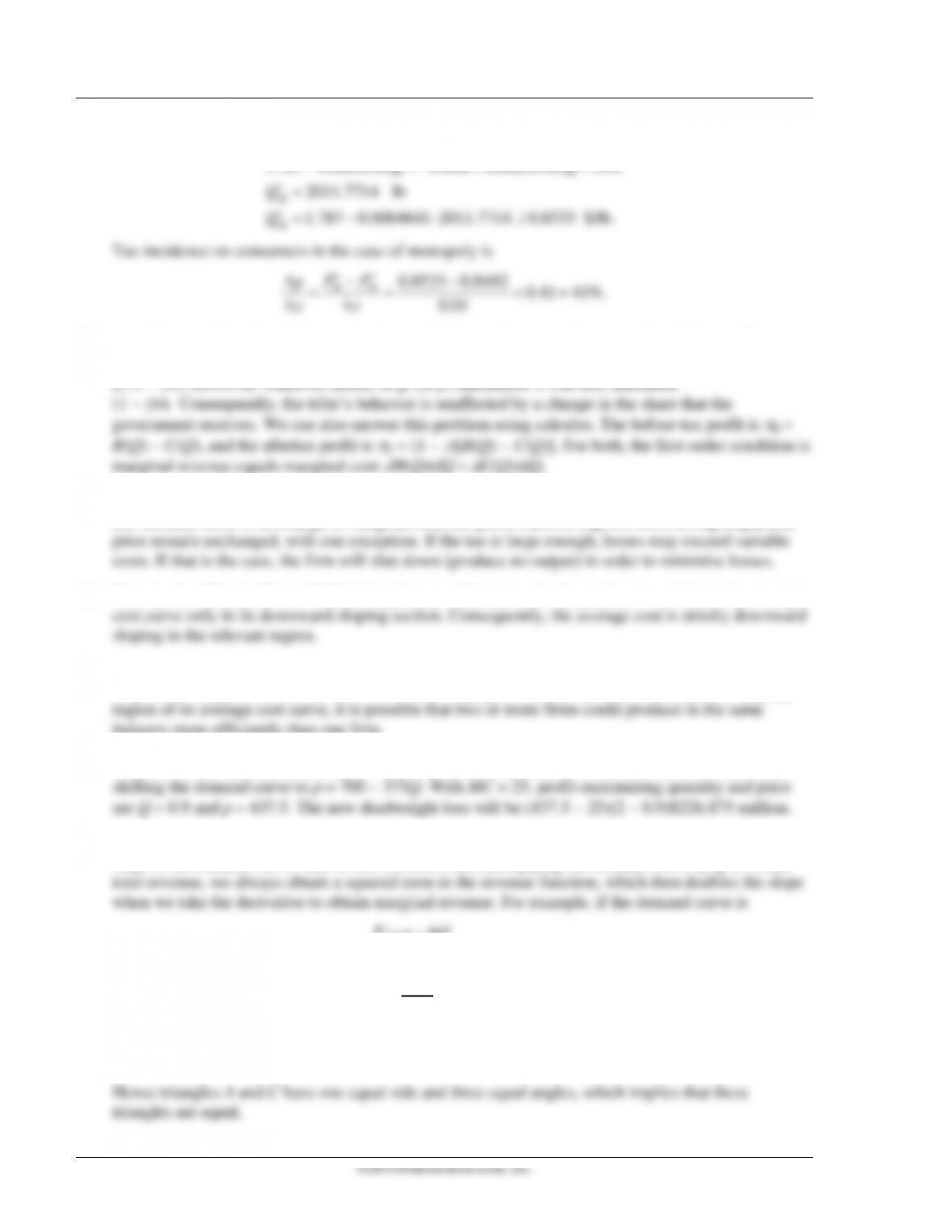
Then
− =−+ +
′=
′=−⋅
1.787 0.0009282 0.496 0.00020165 0.01
2011.7714 lb
1.787 0.0004641 2011.7714 0.8533 $/lb.
M
M
QQ
Q
Q
Tax incidence on consumers in the case of monopoly is
ττ
′−
∆−
= = = ≡
∆∆
*0.8533 0.8492 0.41 41%.
0.01
MM
PP
p
3.4 A profit tax (of less than 100 percent) has no effect on a firm’s profit-maximizing behavior. Suppose
the government’s share of the profit is
β
. Then the firm wants to maximize its after–tax profit, which
3.5 The effect of a franchise tax or lump sum tax on a monopoly is to reduce profits by the amount of the
4.1 Yes. As the “Electric Power Utilities” application illustrates, the demand curve could cut the average
4.2 No. In order for a firm to be a natural monopoly, its production must exhibit economies of scale; that
is, firm’s average cost curve must be downward sloping. If the firm operates in the upward-sloping
4.3 The inverse demand function is p = 775 − 375Q. Imposing a specific tax of $75 will be equivalent to
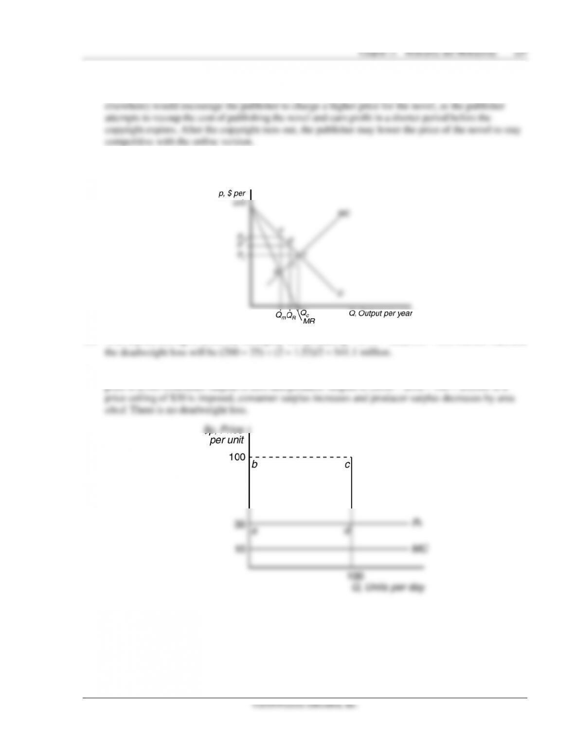
4.4 When the demand curve is linear, the marginal revenue curve will always be linear with twice the
TR = aQ − bQ2
= = − 2.
dTR
MR a bQ
dQ
Because the slope of MR is double of the slope of the linear demand curve, MR curve always crosses
the MC segment in the middle between the y–axis and point
c
e
(see figure in the Botox application).
230 Perloff • Microeconomics: Theory and Applications with Calculus, Third Edition
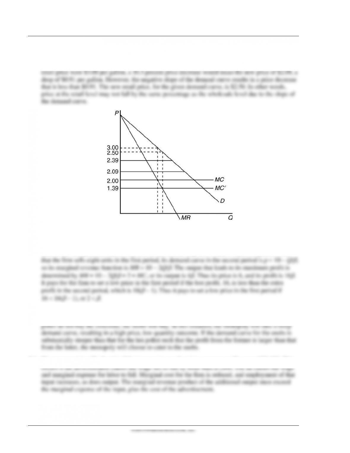
5.4 The wholesale price of milk represents the marginal cost for retailers, who sell to consumers. In
the figure below, suppose prices at the wholesale level fall 30.3 percent from $2.00 to $1.394 per
gallon, or $0.606 per gallon. That is, for retailers, marginal cost shifts from MC to MC′. If the original
6.1 Given that the demand curve is p = 10 − Q, its marginal revenue curve is MR = 10 − 2Q. Thus the
output that maximizes the monopoly’s profit is determined by MR = 10 − 2Q = 2 = MC, or Q* = 4. At
that output level, its price is p* = 6, and its profit is
π
* = 16. If the monopoly chooses to sell eight
units in the first period (it has no incentive to sell more), its price is 2 and it makes no profit. Given
6.2 When the hoi polloi buy the chocolate, the snobs won’t buy. So the monopoly is facing a relatively
flat demand curve, which suggests a low price, high quantity outcome. On the contrary, if the hoi
7.1 The monopsonist will advertise if the increase in preadvertising expense profits exceed $1,000. This
232 Perloff • Microeconomics: Theory and Applications with Calculus, Third Edition
7.6 If a firm has a monopoly in the output market and is a monopsony in the labor market, its profit is
(())() (),π= −pQL QL wLL
where Q(L) is the production function, p(Q)Q is its revenue, and wL—the wage times the number of
workers—is its cost of production. The firm maximizes its profit by setting the derivative of profit
with respect to labor equal to zero (if the second-order condition holds):
() () 0.
+ −−=
dp dQ dw
p QL wL L
dQ dL dL
Rearranging terms in the first–order condition, we find that the maximization condition is that the
marginal revenue product of labor,
1
( ) () 1
ε
==+=+
LL
dp dQ dQ
MRP MR MP p Q L p
dQ dL dL
equals the marginal expenditure,
() ()1
1
()1
η
=+= +
= +
dw L dw
ME wL L wL
dL w dL
wL
where
ε
is the elasticity of demand in the output market and
η
is the supply elasticity of labor.
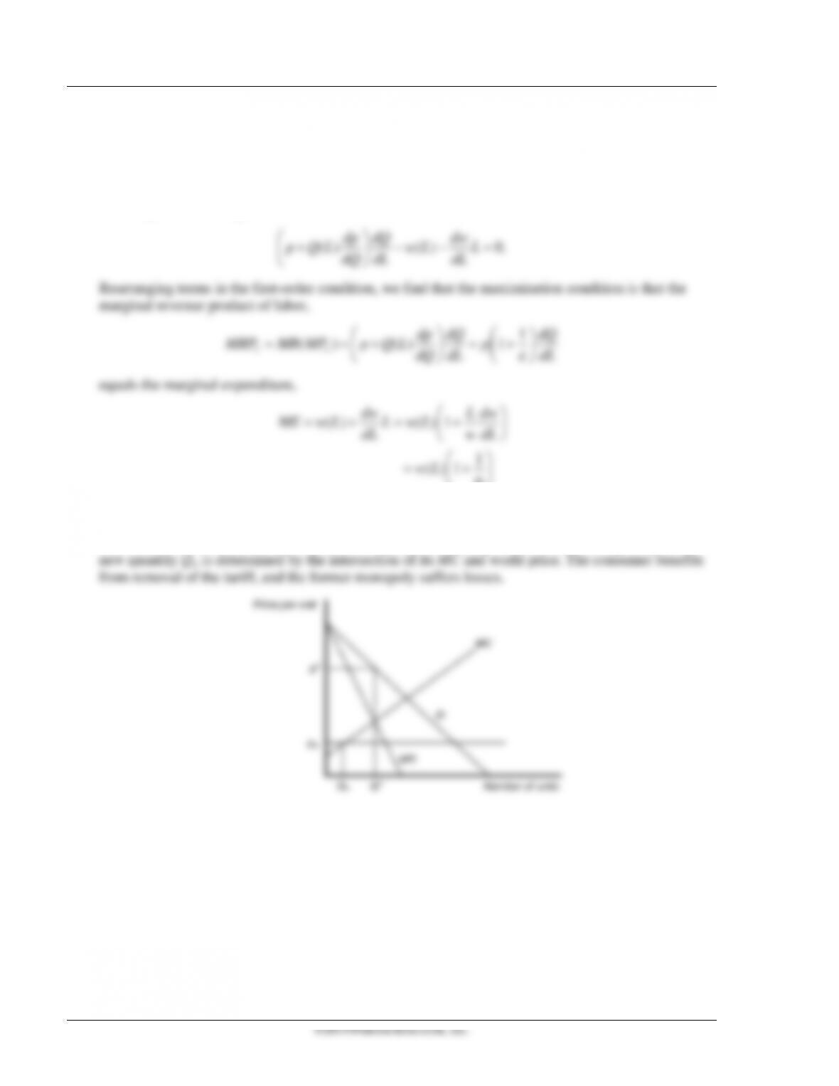
8.1 After the remove of the tariff, the former monopoly will sell its products at the world price pw. The