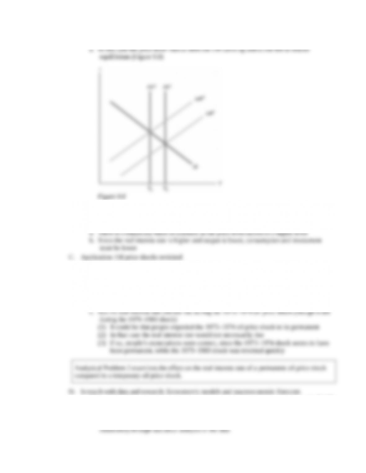
4. Since the FE, IS, and LM curves don’t intersect, the price level adjusts, shifting the LM curve
until a general equilibrium is reached
5. The inflation rate rises temporarily, not permanently
6. Summary: The real wage, employment, and output decline, while the real interest rate and
price level are higher
1. Does the IS-LM model correctly predict the results of an adverse supply shock?
2. The data from the 1973–1974 and 1979–1980 oil price shocks shows the following
a. As discussed in Chapter 3, output, employment, and the real wage declined
b. Consumption fell slightly and investment fell substantially
c. Inflation surged temporarily
d. All the above results are consistent with the theory
1. Many models that are used for macroeconomic research and analysis are based on the IS-LM
model
2. There are three major steps in using an economic model for forecasting
a. An econometric model estimates the parameters of the model (slopes, intercepts,
elasticities) through statistical analysis of the data
3. The Federal Reserve Board’s FRB/US model, introduced in 1996, improves on the old model
by better handling of expectations, improved modeling of reactions to shocks, and use of
4. The FRB/US model is the workhorse for policy analysis by the Fed’s staff economists
5. Board of Governor’s staff adjust the FRB/US forecasts with their judgment; the subsequent
forecasts reported in the Greenbook have been found to be superior to private-sector
forecasts
Theoretical Application
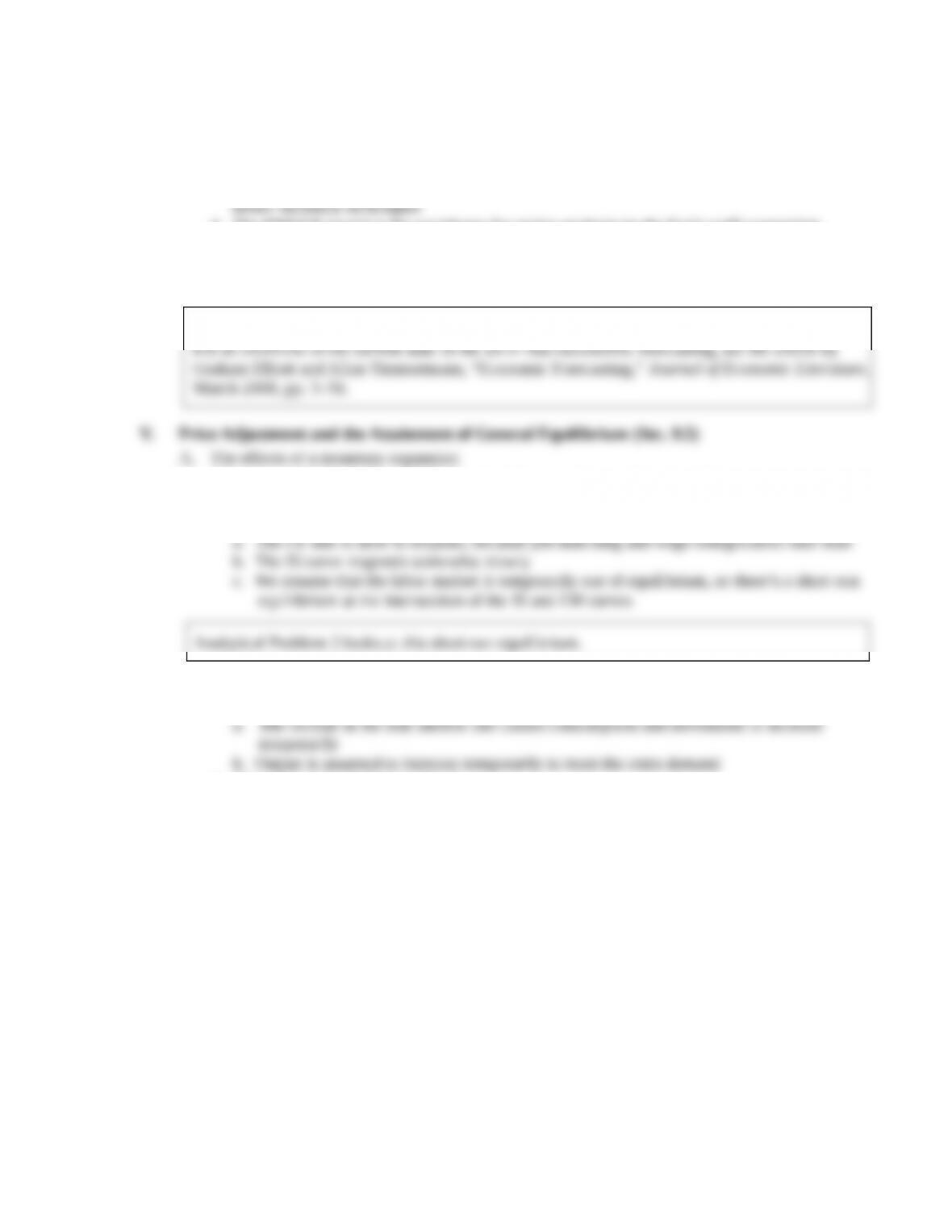
1. An increase in money supply shifts the LM curve down and to the right
2. Because financial markets respond most quickly to changes in economic conditions, the asset
market responds to the disequilibrium
3. The increase in the money supply causes people to try to get rid of excess money balances by
buying assets, driving the real interest rate down
4. The adjustment of the price level
a. Since the demand for goods exceeds firms’ desired supply of goods, firms raise prices
b. The rise in the price level causes the LM curve to shift up
c. The price level continues to rise until the LM curve intersects with the FE line and the IS
curve at general equilibrium (Figure 9.9)
5. Trend money growth and inflation
a. This analysis also handles the case in which the money supply is growing continuously
b. If both the money supply and price level rise by the same proportion, there is no change
in the real money supply, and the LM curve doesn’t shift
c. If the money supply grew faster than the price level, the LM curve would shift down and
1. There are two key questions in the debate between classical and Keynesian approaches
a. How rapidly does the economy reach general equilibrium?
2. Price adjustment and the self-correcting economy
a. The economy is brought into general equilibrium by adjustment of the price level
b. The speed at which this adjustment occurs is much debated
c. Classical economists see rapid adjustment of the price level
3. Monetary neutrality
a. Money is neutral if a change in the nominal money supply changes the price level
proportionately but has no effect on real variables
b. The classical view is that a monetary expansion affects prices quickly with at most a
1. The two models are equivalent
2. Depending on the issue, one model or the other may prove more useful
a. IS-LM relates the real interest rate to output
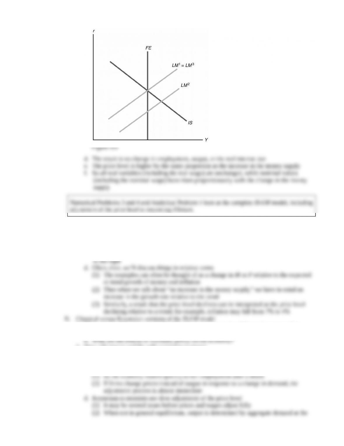
1. The AD curve shows the relationship between the quantity of goods demanded and the price
level when the goods market and asset market are in equilibrium
a. So the AD curve represents the price level and output level at which the IS and LM curves
intersect (Figure 9.10)
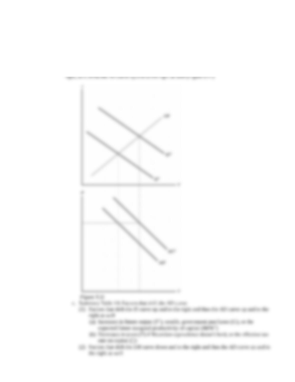
2. Factors that shift the AD curve
a. Any factor that causes the intersection of the IS and LM curves to shift to the left causes the
AD curve to shift down and to the left; any factor causing the IS–LM intersection to shift to the
right causes the AD curve to shift up and to the right
b. For example, a temporary increase in government purchases shifts the IS curve up and to the
1. The aggregate supply curve shows the relationship between the price level and the aggregate
amount of output that firms supply
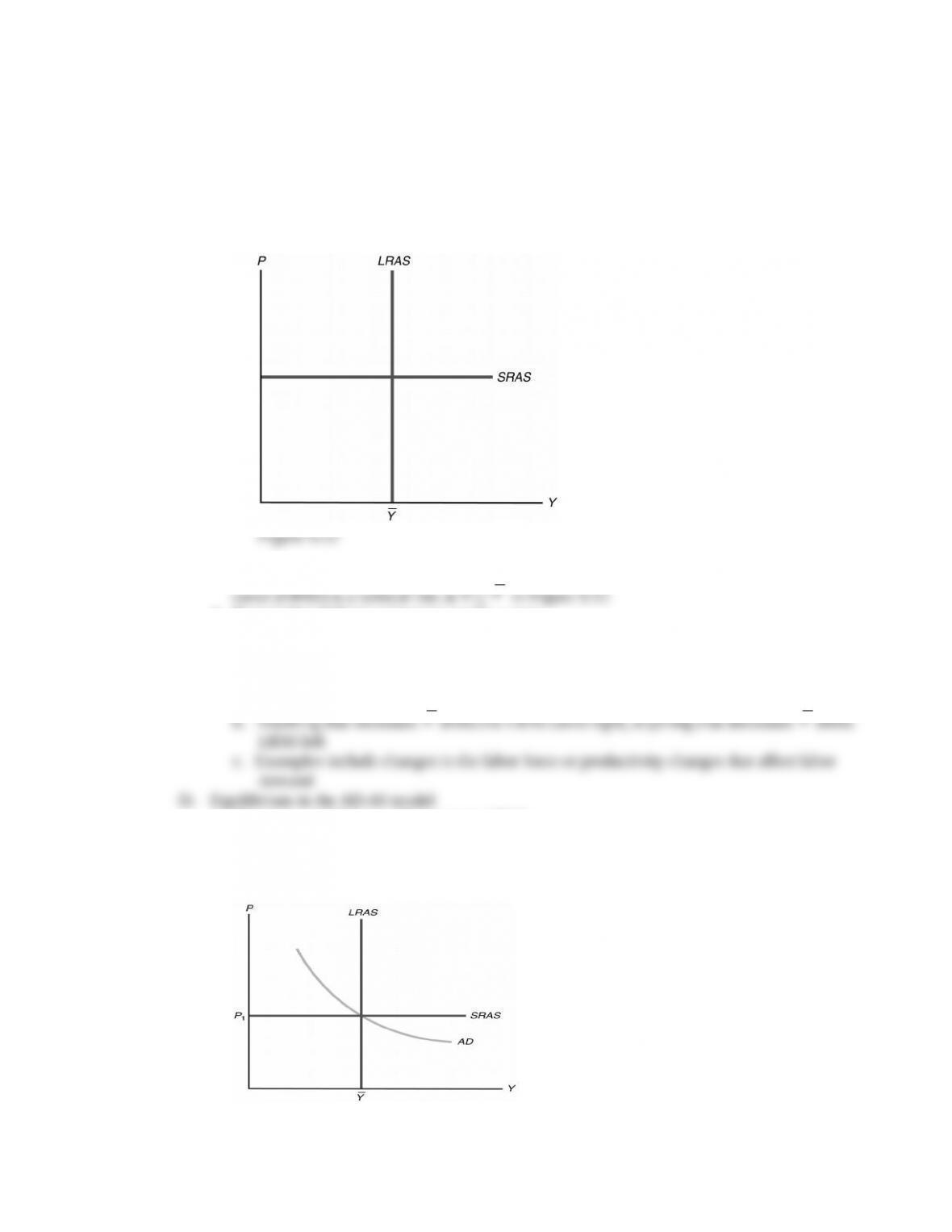
2. In the short run, prices remain fixed, so firms supply whatever output is demanded
a. The short-run aggregate supply curve is horizontal (Figure 9.12)
3. Full-employment output isn’t affected by the price level, so the long-run aggregate supply
curve (LRAS) is a vertical line at Y
Y
in Figure 9.12
4. Factors that shift the aggregate supply curves
a. The SRAS curve shifts whenever firms change their prices in the short run
(1) Factors like increased costs of producing goods lead firms to increase prices, shifting
SRAS up
(2) Factors leading to reduced prices shift SRAS down
1. Short-run equilibrium: AD intersects SRAS
2. Long-run equilibrium: AD intersects LRAS
a. Also called general equilibrium
b. AD, LRAS, and SRAS all intersect at same point (Figure 9.13)
Figure 9.13
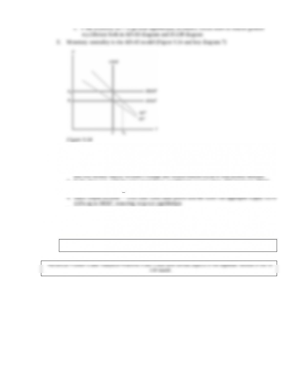
1. Suppose the economy begins in general equilibrium, but then the money supply is increased
by 10%
2. This shifts the AD curve upward by 10% (from AD1 to AD2) because to maintain the
aggregate quantity demanded at a given level, the price level would have to rise by 10% so
3. In the short run, with the price level fixed, equilibrium occurs where AD2 intersects SRAS1,
with a higher level of output
,Y
5. The result is a higher price level—higher by 10%
6. Money is neutral in the long run, as output is unchanged
F. The key question is: How long does it take to get from the short run to the long run?
1. The answer to this question is what separates classicals from Keynesians
Numerical Problem 5 illustrates the effects of monetary and fiscal policy using the model.
3. The Federal Reserve Board’s FRB/US model, introduced in 1996, improves on the old model
by better handling of expectations, improved modeling of reactions to shocks, and use of
4. The FRB/US model is the workhorse for policy analysis by the Fed’s staff economists
5. Board of Governor’s staff adjust the FRB/US forecasts with their judgment; the subsequent
forecasts reported in the Greenbook have been found to be superior to private-sector
forecasts
Theoretical Application
1. An increase in money supply shifts the LM curve down and to the right
2. Because financial markets respond most quickly to changes in economic conditions, the asset
market responds to the disequilibrium
3. The increase in the money supply causes people to try to get rid of excess money balances by
buying assets, driving the real interest rate down
4. The adjustment of the price level
a. Since the demand for goods exceeds firms’ desired supply of goods, firms raise prices
b. The rise in the price level causes the LM curve to shift up
c. The price level continues to rise until the LM curve intersects with the FE line and the IS
curve at general equilibrium (Figure 9.9)
5. Trend money growth and inflation
a. This analysis also handles the case in which the money supply is growing continuously
b. If both the money supply and price level rise by the same proportion, there is no change
in the real money supply, and the LM curve doesn’t shift
c. If the money supply grew faster than the price level, the LM curve would shift down and
1. There are two key questions in the debate between classical and Keynesian approaches
a. How rapidly does the economy reach general equilibrium?
2. Price adjustment and the self-correcting economy
a. The economy is brought into general equilibrium by adjustment of the price level
b. The speed at which this adjustment occurs is much debated
c. Classical economists see rapid adjustment of the price level
3. Monetary neutrality
a. Money is neutral if a change in the nominal money supply changes the price level
proportionately but has no effect on real variables
b. The classical view is that a monetary expansion affects prices quickly with at most a
1. The two models are equivalent
2. Depending on the issue, one model or the other may prove more useful
a. IS-LM relates the real interest rate to output
1. The AD curve shows the relationship between the quantity of goods demanded and the price
level when the goods market and asset market are in equilibrium
a. So the AD curve represents the price level and output level at which the IS and LM curves
intersect (Figure 9.10)
2. Factors that shift the AD curve
a. Any factor that causes the intersection of the IS and LM curves to shift to the left causes the
AD curve to shift down and to the left; any factor causing the IS–LM intersection to shift to the
right causes the AD curve to shift up and to the right
b. For example, a temporary increase in government purchases shifts the IS curve up and to the
1. The aggregate supply curve shows the relationship between the price level and the aggregate
amount of output that firms supply
2. In the short run, prices remain fixed, so firms supply whatever output is demanded
a. The short-run aggregate supply curve is horizontal (Figure 9.12)
3. Full-employment output isn’t affected by the price level, so the long-run aggregate supply
curve (LRAS) is a vertical line at Y
Y
in Figure 9.12
4. Factors that shift the aggregate supply curves
a. The SRAS curve shifts whenever firms change their prices in the short run
(1) Factors like increased costs of producing goods lead firms to increase prices, shifting
SRAS up
(2) Factors leading to reduced prices shift SRAS down
1. Short-run equilibrium: AD intersects SRAS
2. Long-run equilibrium: AD intersects LRAS
a. Also called general equilibrium
b. AD, LRAS, and SRAS all intersect at same point (Figure 9.13)
Figure 9.13
1. Suppose the economy begins in general equilibrium, but then the money supply is increased
by 10%
2. This shifts the AD curve upward by 10% (from AD1 to AD2) because to maintain the
aggregate quantity demanded at a given level, the price level would have to rise by 10% so
3. In the short run, with the price level fixed, equilibrium occurs where AD2 intersects SRAS1,
with a higher level of output
,Y
5. The result is a higher price level—higher by 10%
6. Money is neutral in the long run, as output is unchanged
F. The key question is: How long does it take to get from the short run to the long run?
1. The answer to this question is what separates classicals from Keynesians
Numerical Problem 5 illustrates the effects of monetary and fiscal policy using the model.