
Chapter 9
The IS–LM/AD-AS Model: A General
Framework for Macroeconomic Analysis
Learning Objectives
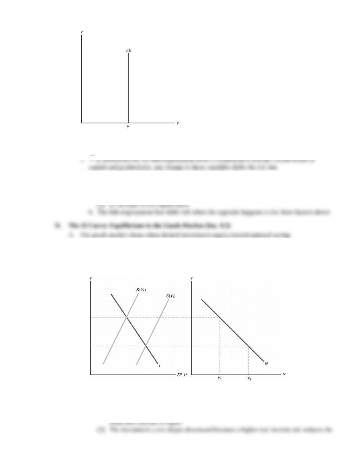
1. Describe the factors that explain the full-employment (FE) line (Sec. 9.1)
2. Discuss the factors that affect the IS curve, which represents equilibrium in the goods
market (Sec. 9.2)
3. Discuss the factors that affect the LM curve, which represents equilibrium in the asset
market (Sec. 9.3)
4. Describe the conditions necessary for general equilibrium using the IS-LM model (Sec.
9.4)
5. Discuss the role of price adjustment in achieving general equilibrium (Sec. 9.5)
6. Explain the fundamentals and implications of the AD-AS model (Sec. 9.6)
II. Notes to Seventh Edition Users
A. This chapter has not changed significantly
Teaching Notes
I. The FE Line: Equilibrium in the Labor Market (Sec. 9.1)
A. In the discussion of the labor market in Chapter 3, we showed how equilibrium in the labor
market leads to employment at its full-employment level
N
and output at
Y
B. If we plot output against the real interest rate, we get a vertical line at Y
Y
, since labor market
equilibrium is unaffected by changes in the real interest rate (Figure 9.1)
2. Summary Table 11 lists the factors that shift the full-employment line
a. The full-employment line shifts right because of
(1) a beneficial supply shock
(2) an increase in labor supply
1. Adjustments in the real interest rate bring about equilibrium
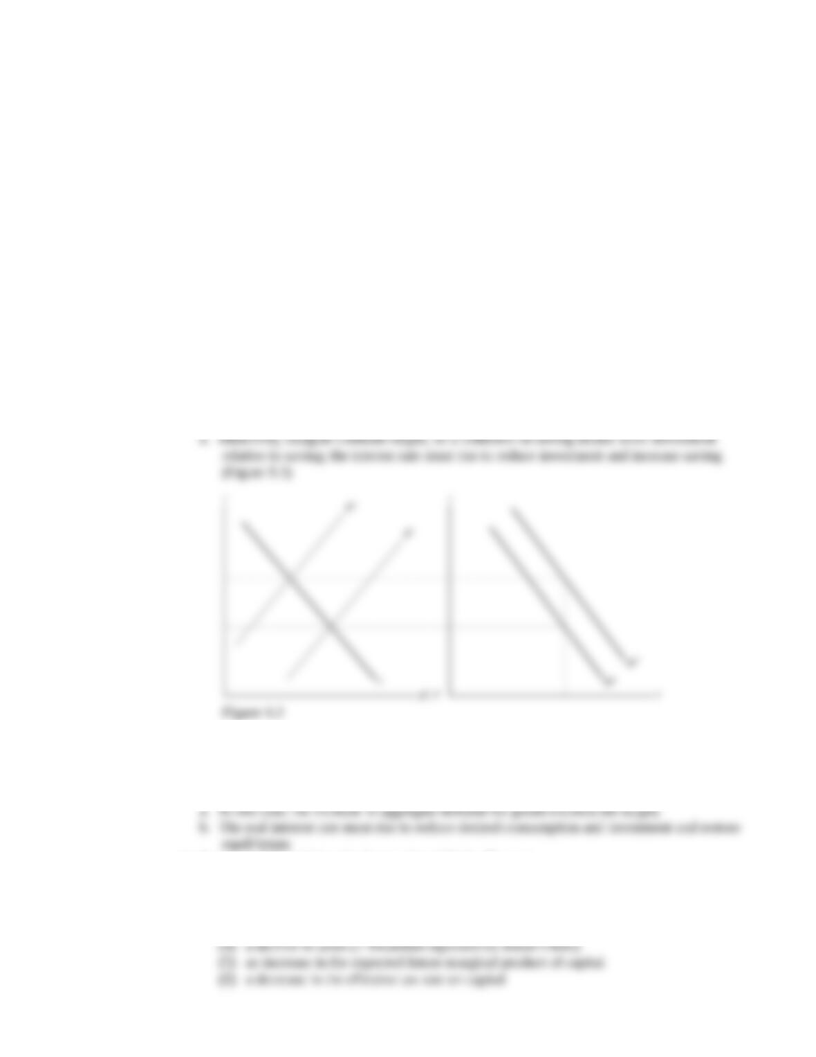
2. For any level of output Y, the IS curve shows the real interest rate r for which the goods
market is in equilibrium
3. Derivation of the IS curve from the saving-investment diagram (Figure 9.2)
Figure 9.2
a. Key features
(1) The saving curve slopes upward because a higher real interest rate increases saving
(2) An increase in output shifts the saving curve to the right, because people save more
1. Any change that reduces desired national saving relative to desired investment shifts the IS
curve up and to the right
2. Similarly, a change that increases desired national saving relative to desired investment shifts
the IS curve down and to the left
3. An alternative way of stating this is that a change that increases aggregate demand for goods
shifts the IS curve up and to the right
4. Summary Table 12 lists the factors that shift the IS curve
a. The IS curve shifts up and to the right because of
(1) an increase in expected future output
(2) an increase in wealth
(3) a temporary increase in government purchases
1. The price of a nonmonetary asset is inversely related to its interest rate or yield
a. Example: A bond pays $10,000 in one year; its current price is $9615, and its interest rate
is 4%, since ($10,000 $9615)/$9615 0.04 4%
b. If the price of the bond in the market were to fall to $9524, its yield would rise to 5%,
2. For a given level of expected inflation, the price of a nonmonetary asset is inversely related
to the real interest rate
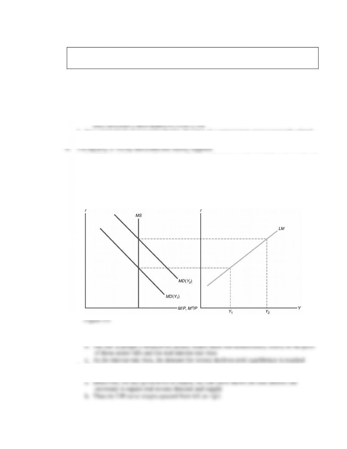
1. Equilibrium in the asset market requires that the real money supply equal the real quantity of
money demanded
2. Real money supply is determined by the central bank and isn’t affect by the real interest rate
3. Real money demand falls as the real interest rate rises
4. Real money demand rises as the level of output rises
5. The LM curve (Figure 9.4) is derived by plotting real money demand for different levels of
output and looking at the resulting equilibrium
6. By what mechanism is equilibrium restored?
a. Starting at equilibrium, suppose output rises, so real money demand increases
7. The LM curve shows the combinations of the real interest rate and output that clear the
asset market
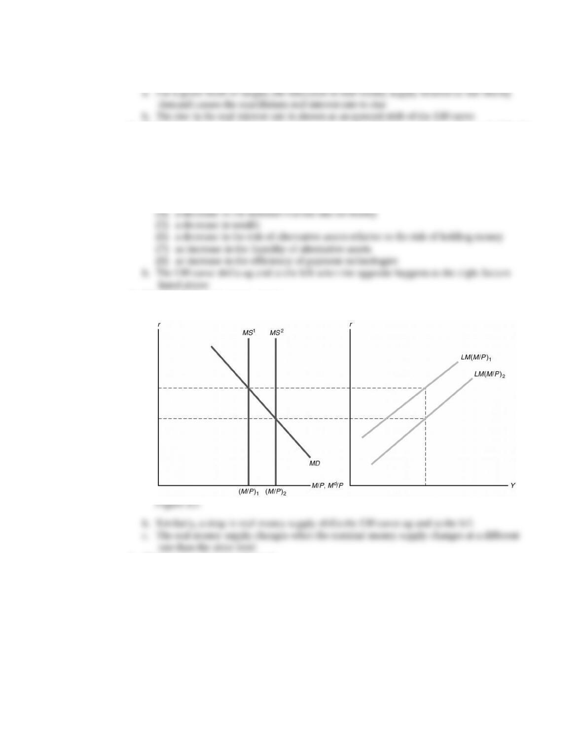
1. Any change that reduces real money supply relative to real money demand shifts the LM
curve up
2. Similarly, a change that increases real money supply relative to real money demand shifts the
LM curve down and to the right
3. Summary Table 13 lists the factors that shift the LM curve
a. The LM curve shifts down and to the right because of
(1) an increase in the nominal money supply
(2) a decrease in the price level
(3) an increase in expected inflation
4. Changes in the real money supply
a. An increase in the real money supply shifts the LM curve down and to the right (Figure 9.5)
5. Changes in real money demand
a. An increase in real money demand shifts the LM curve up and to the left (Figure 9.6)
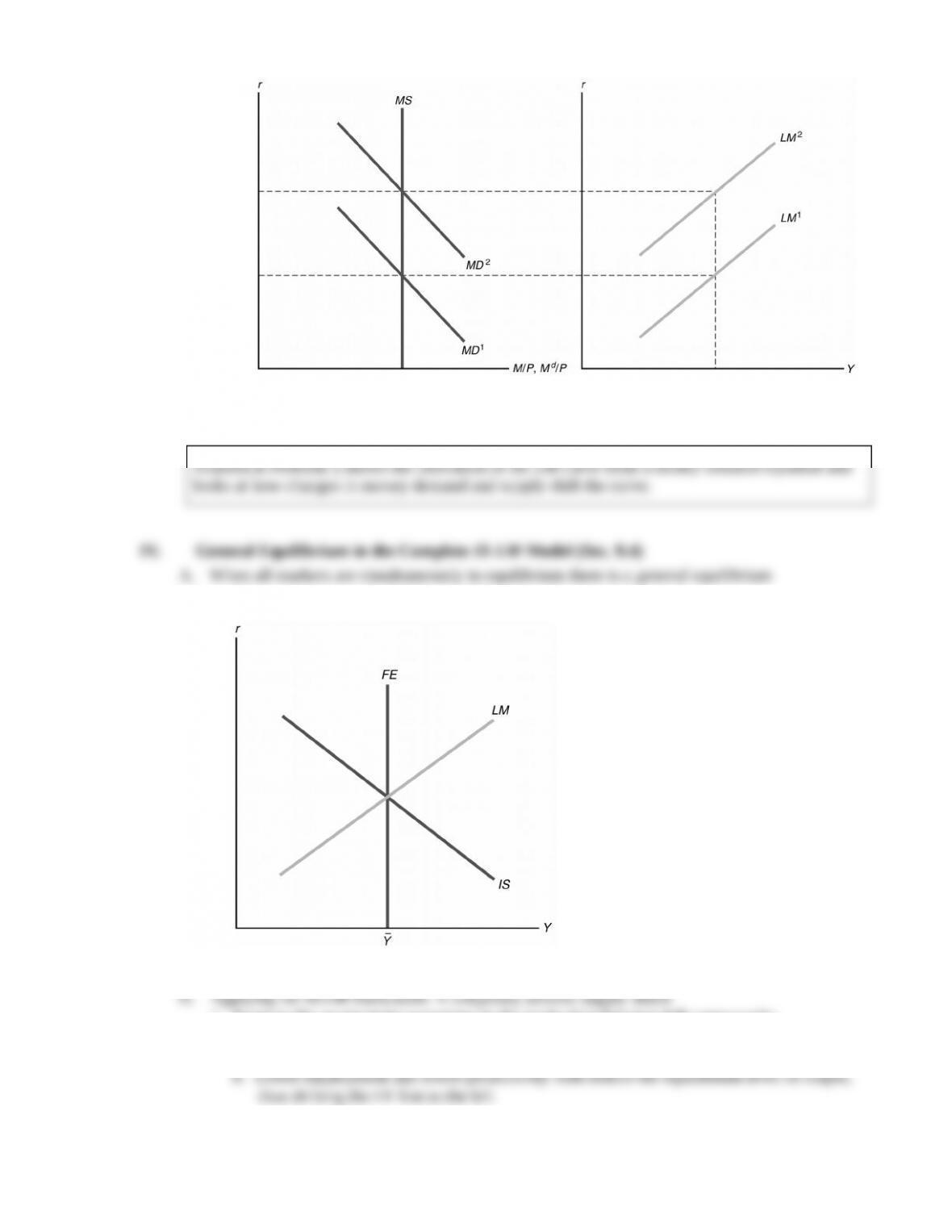
Figure 9.6
b. Similarly, a drop in real money demand shifts the LM curve down and to the right
1. This occurs where the FE, IS, and LM curves intersect (Figure 9.7)
Figure 9.7
1. Suppose the productivity parameter in the production function falls temporarily
2. The supply shock reduces the marginal productivity of labor, hence labor demand
a. With lower labor demand, the equilibrium real wage and employment fall

3. There’s no effect of a temporary supply shock on the IS or LM curves
2. Summary Table 11 lists the factors that shift the full-employment line
a. The full-employment line shifts right because of
(1) a beneficial supply shock
(2) an increase in labor supply
1. Adjustments in the real interest rate bring about equilibrium
2. For any level of output Y, the IS curve shows the real interest rate r for which the goods
market is in equilibrium
3. Derivation of the IS curve from the saving-investment diagram (Figure 9.2)
Figure 9.2
a. Key features
(1) The saving curve slopes upward because a higher real interest rate increases saving
(2) An increase in output shifts the saving curve to the right, because people save more
1. Any change that reduces desired national saving relative to desired investment shifts the IS
curve up and to the right
2. Similarly, a change that increases desired national saving relative to desired investment shifts
the IS curve down and to the left
3. An alternative way of stating this is that a change that increases aggregate demand for goods
shifts the IS curve up and to the right
4. Summary Table 12 lists the factors that shift the IS curve
a. The IS curve shifts up and to the right because of
(1) an increase in expected future output
(2) an increase in wealth
(3) a temporary increase in government purchases
1. The price of a nonmonetary asset is inversely related to its interest rate or yield
a. Example: A bond pays $10,000 in one year; its current price is $9615, and its interest rate
is 4%, since ($10,000 $9615)/$9615 0.04 4%
b. If the price of the bond in the market were to fall to $9524, its yield would rise to 5%,
2. For a given level of expected inflation, the price of a nonmonetary asset is inversely related
to the real interest rate
1. Equilibrium in the asset market requires that the real money supply equal the real quantity of
money demanded
2. Real money supply is determined by the central bank and isn’t affect by the real interest rate
3. Real money demand falls as the real interest rate rises
4. Real money demand rises as the level of output rises
5. The LM curve (Figure 9.4) is derived by plotting real money demand for different levels of
output and looking at the resulting equilibrium
6. By what mechanism is equilibrium restored?
a. Starting at equilibrium, suppose output rises, so real money demand increases
7. The LM curve shows the combinations of the real interest rate and output that clear the
asset market
1. Any change that reduces real money supply relative to real money demand shifts the LM
curve up
2. Similarly, a change that increases real money supply relative to real money demand shifts the
LM curve down and to the right
3. Summary Table 13 lists the factors that shift the LM curve
a. The LM curve shifts down and to the right because of
(1) an increase in the nominal money supply
(2) a decrease in the price level
(3) an increase in expected inflation
4. Changes in the real money supply
a. An increase in the real money supply shifts the LM curve down and to the right (Figure 9.5)
5. Changes in real money demand
a. An increase in real money demand shifts the LM curve up and to the left (Figure 9.6)
Figure 9.6
b. Similarly, a drop in real money demand shifts the LM curve down and to the right
1. This occurs where the FE, IS, and LM curves intersect (Figure 9.7)
Figure 9.7
1. Suppose the productivity parameter in the production function falls temporarily
2. The supply shock reduces the marginal productivity of labor, hence labor demand
a. With lower labor demand, the equilibrium real wage and employment fall
3. There’s no effect of a temporary supply shock on the IS or LM curves