1. Classical economists see little need for government action
1. NBER maintains the business cycle chronology—a detailed history of business cycles
2. NBER sponsors business cycle studies
Data Application
A major compendium of studies on the business cycle was produced by the NBER in 1986, The
American Business Cycle: Continuity and Change, edited by Robert J. Gordon, Chicago:
University of Chicago Press. It contains general discussions of the then-current state of
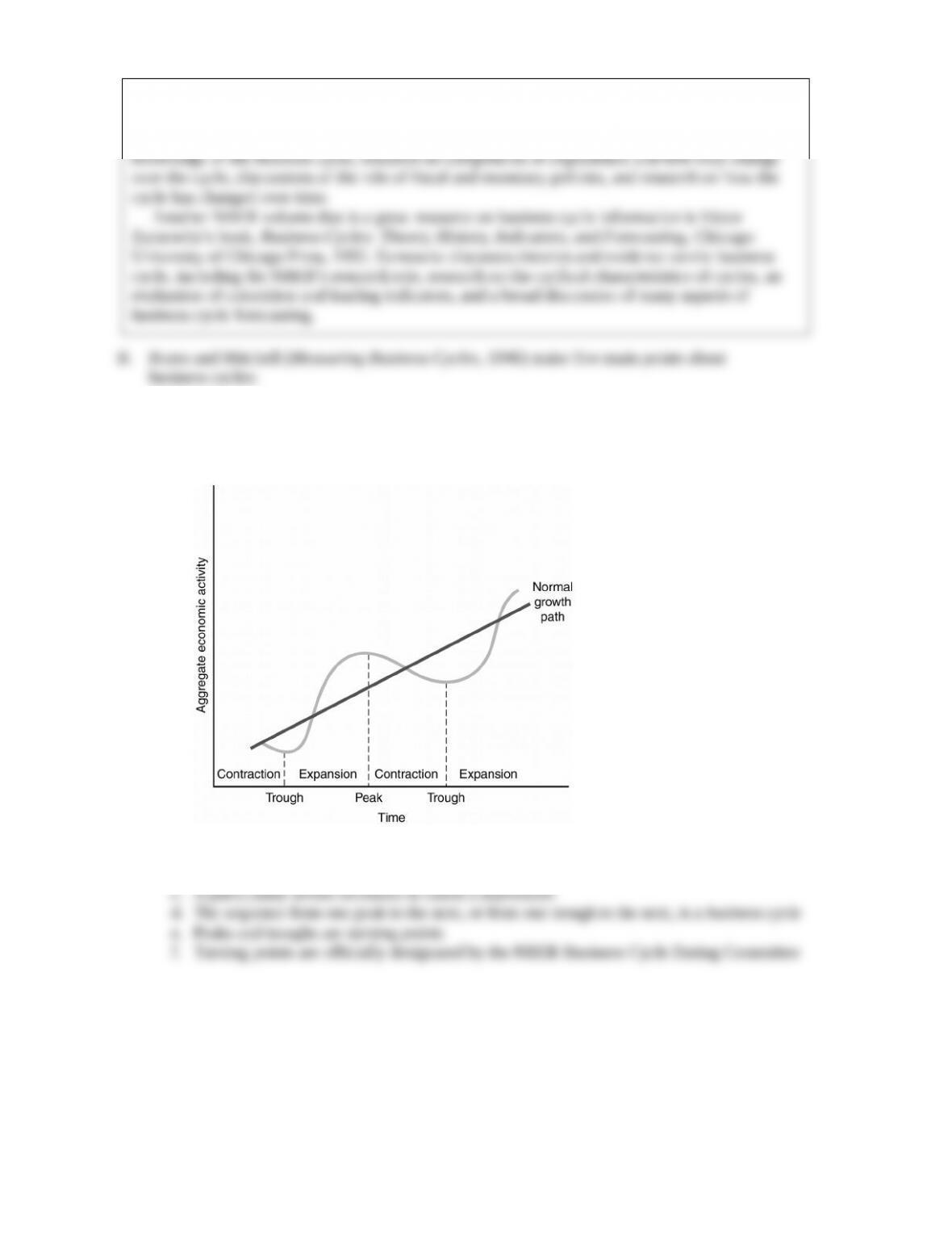
1. Business cycles are fluctuations of aggregate economic activity, not a specific variable
2. There are expansions and contractions
a. Aggregate economic activity declines in a contraction or recession until it reaches a
trough (Figure 8.1)
Figure 8.1
b. Then activity increases in an expansion or boom until it reaches a peak

3. Economic variables show comovement—they have regular and predictable patterns of
behavior over the course of the business cycle
4. The business cycle is recurrent, but not periodic
a. Recurrent means the pattern of contraction–trough–expansion–peak occurs again and again
5. The business cycle is persistent
a. Declines are followed by further declines; growth is followed by more growth
b. Because of persistence, forecasting turning points is quite important
Theoretical Application
Should we even care about the business cycle? Robert Lucas doesn’t think so. In his provocative
3–18. They provide a basic set of facts (viewed through the lens of RBC theory) about the
movement of economic variables over the business cycle. They also suggest that inflation is
1. Recessions were common from 1865 to 1917, with 338 months of contraction and
382 months of expansion [compared with 642 months of expansion and 122 months of
contraction from 1945 to 2009]
2. The longest contraction on record was 65 months, from October 1873 to March 1879
C. The Great Depression and World War II
1. The worst economic contraction was the Great Depression of the 1930s
a. Real GDP fell nearly 30% from the peak in August 1929 to the trough in March 1933
b. The unemployment rate rose from 3% to nearly 25%
c. Thousands of banks failed, the stock market collapsed, many farmers went bankrupt, and
international trade was halted
2. The Great Depression ended with the start of World War II
a. Wartime production brought the unemployment rate below 2%
1. From 1945 to 1970 there were five mild contractions
2. A very long expansion (106 months, from February 1961 to December 1969) made some
economists think the business cycle was dead
3. But the OPEC oil shock of 1973 caused a sharp recession, with real GDP declining 3%, the
unemployment rate rising to 9%, and inflation rising to over 10%
4. The 1981–1982 recession was also severe, with the unemployment rate over 11%, but
inflation declining from 11% to less than 4%
5. The 1990–1991 recession was mild and short, but the recovery was slow and erratic
E. The long boom
1. From 1982 to 2001, there was only one brief recession, from July 1990 to March 1991,
which was not very severe
2. The volatility of many macroeconomic variables declined sharply, so the Long Boom was the
first part of the period known as the Great Moderation
1. The longest and deepest recession since the Great Depression began in December 2007
a. The Great Recession began with a housing crisis (described in Chapter 7)
2. The unemployment rose above 10% for the first time since 1982 and the Fed reduced
interest rates to near zero
3. Economic growth was sluggish even after the recession ended in 2009
Data Application
1. Economists believed that business cycles weren’t as bad after World War II as they were
before
2. The average contraction before 1929 lasted 21 months compared to 11 months after 1945
3. The average expansion before 1929 lasted 25 months compared to 50 months after 1945
4. Romer’s 1986 article sparked a strong debate, as it argued that pre-1929 data was not
measured well, and that business cycles weren’t that bad before 1929
5. New research has focused on the reasons for the decline in the volatility of U.S. output
a. Stock and Watson’s research showed that the decline came from a sharp drop in volatility
around 1984 for many economic variables; dubbed the Great Moderation
b. A plot of real GDP growth (text Figure 8.2) shows that the quarterly growth rate of GDP
was more stable after 1984
6. After showing that many theories for the reduced volatility in output were not convincing,
Stock and Watson found three factors that were important
30% of the reduction in the volatility of output
d. The remaining reduction in output’s volatility remains unexplained–some unknown form
7. It is not yet clear if the Great Recession implies that the Great Moderation has ended
Data Application
Frank Diebold and Glenn Rudebusch argue that although the debate between Romer and others
about the volatility of business cycles before 1929 compared to after 1945 is unsettled, there is clear
1. What direction does a variable move relative to aggregate economic activity?
a. Procyclical: in the same direction
2. What is the timing of a variable’s movements relative to aggregate economic activity?
a. Leading: in advance
b. Coincident: at the same time
c. Lagging: after
1. Procyclical
a. Coincident: industrial production, consumption, business fixed investment, and employment
b. Leading: residential investment, inventory investment, average labor productivity, money
growth, and stock prices
2. Countercyclical: unemployment (timing is unclassified)
3. Acyclical: real interest rates (timing is not designated)
4. Volatility: durable goods production is more volatile than nondurable goods and services;
investment spending is more volatile than consumption
5. Application: The Job Finding Rate and the Job Loss Rate
a. The probability that someone finds or loses a job in a given month changes over time
b. The job finding rate is the probability that someone who is unemployed will find a job
during the month, but that probability declines in recessions and increases in expansions
(text Figure 8.8)
1. The cyclical behavior of key economic variables in other countries is similar to that in the
United States
2. Major industrial countries frequently have recessions and expansions at about the same time
3. Text Figure 8.13 illustrates common cycles for Japan, Canada, the United States, France,
Germany, and the United Kingdom
4. In addition, each economy faces small fluctuations that aren’t shared with other countries
Data Application
1. Coincident indexes are designed to help figure out the current state of the economy, while
leading indicators are designed to help predict peaks and troughs
2. The first index was developed by Mitchell and Burns of the NBER in the 1930s
3. The CFNAI is a coincident index produced by the Federal Reserve Bank of Chicago based on
85 macroeconomic variables; it is a coincident index that turns significantly negative in
recessions (text Figure 8.14)
4. The ADS Business Conditions Index is a coincident index based on variables of different
frequencies (text Figure 8.15)
5. The CFNAI and ADS index perform similarly; the ADS is available more frequently but
doesn’t have a long track record
6. The Conference Board produces an index of leading economic indicators; a decline in the
index for two or three months in a row warns of recession danger
7. Problems with the leading indicators
a. Data are available promptly, but often revised later, so the index may give
8. Research by Diebold and Rudebusch showed that the index does not help forecast industrial
production in real time
9. In real time, the index sometimes gave no warning of recessions
a. The index gave no advance warning of the recession that began in December 1970
10. After the fact, the index of leading indicators is revised and appears to have predicted the
recessions well
11. Stock and Watson attempted to improve the index by creating some new indexes based on
newer statistical methods, but the results were disappointing as the new index failed to
12. Because recessions may be caused by sudden shocks, the search for a good index of leading
indicators may be fruitless
1. Output varies over the seasons: highest in the fourth quarter, lowest in the first quarter

2. Most economic data is seasonally adjusted to remove regular seasonal movements
3. Barsky and Miron’s 1989 study shows that the movements of variables across the seasons are
similar to the movements of variables over the business cycle
Data Application
A further discovery made by Barsky and Miron in looking at the seasonal cycle is surprising:
4. If the seasonal cycle is like the business cycle, and the seasonal cycle represents desirable
responses to various factors (Christmas, the weather) for which government intervention is
inappropriate, should government intervention be used to smooth out the business cycle?
Policy Application
Some economists have gone so far as far as to challenge the need for the Fed to change the
1. 2 major components of business cycle theories
a. A description of the shocks
2. 2 major business cycle theories
a. classical theory
3. Study both theories in aggregate demand-aggregate supply (AD-AS) framework
B. Aggregate demand and aggregate supply: a brief introduction
1. The model (along with the building block IS-LM model) will be developed in chapters 9–11
2. The model has 3 main components; all plotted in (P, Y) space
a. aggregate demand curve
3. Aggregate demand curve
a. Shows quantity of goods and services demanded (Y) for any price level (P)
b. Higher P means less aggregate demand (lower Y), so the aggregate demand curve slopes
downward; reasons why discussed in chapter 9
4. Aggregate supply curve
a. The aggregate supply curve shows how much output producers are willing to supply at
any given price level
b. The short-run aggregate supply curve is horizontal; prices are fixed in the short run
c. The long-run aggregate supply curve is vertical at the full-employment level of output
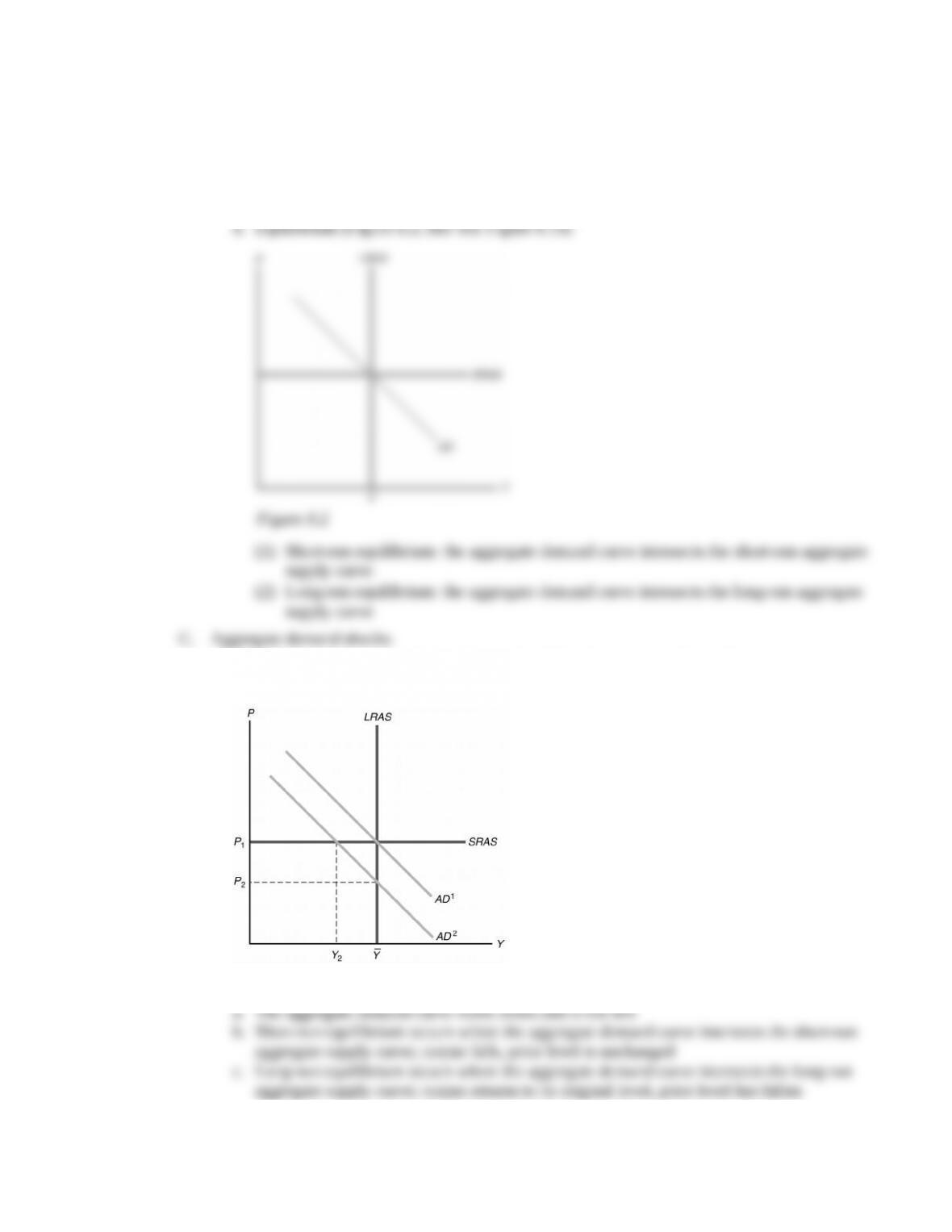
1. An aggregate demand shock is a change that shifts the aggregate demand curve
2. Example: a negative aggregate demand shock (Figure 8.3; like text Figure 8.17)
Figure 8.3

3. How long does it take to get to the long run?
a. Classical theory: prices adjust rapidly
(1) So recessions are short-lived
(2) No need for government intervention
1. Classicals view aggregate supply shocks as the main cause of fluctuations in output
a. An aggregate supply shock is a shift of the long-run aggregate supply curve
2. Example: a negative aggregate supply shock (Figure 8.4, like text Figure 8.18)
Figure 8.4
1
1
1
3. Keynesians also recognize the importance of supply shocks; their views are discussed further
in chapter 11
A major compendium of studies on the business cycle was produced by the NBER in 1986, The
American Business Cycle: Continuity and Change, edited by Robert J. Gordon, Chicago:
University of Chicago Press. It contains general discussions of the then-current state of
1. Business cycles are fluctuations of aggregate economic activity, not a specific variable
2. There are expansions and contractions
a. Aggregate economic activity declines in a contraction or recession until it reaches a
trough (Figure 8.1)
Figure 8.1
b. Then activity increases in an expansion or boom until it reaches a peak
3. Economic variables show comovement—they have regular and predictable patterns of
behavior over the course of the business cycle
4. The business cycle is recurrent, but not periodic
a. Recurrent means the pattern of contraction–trough–expansion–peak occurs again and again
5. The business cycle is persistent
a. Declines are followed by further declines; growth is followed by more growth
b. Because of persistence, forecasting turning points is quite important
Theoretical Application
Should we even care about the business cycle? Robert Lucas doesn’t think so. In his provocative
3–18. They provide a basic set of facts (viewed through the lens of RBC theory) about the
movement of economic variables over the business cycle. They also suggest that inflation is
1. Recessions were common from 1865 to 1917, with 338 months of contraction and
382 months of expansion [compared with 642 months of expansion and 122 months of
contraction from 1945 to 2009]
2. The longest contraction on record was 65 months, from October 1873 to March 1879
C. The Great Depression and World War II
1. The worst economic contraction was the Great Depression of the 1930s
a. Real GDP fell nearly 30% from the peak in August 1929 to the trough in March 1933
b. The unemployment rate rose from 3% to nearly 25%
c. Thousands of banks failed, the stock market collapsed, many farmers went bankrupt, and
international trade was halted
2. The Great Depression ended with the start of World War II
a. Wartime production brought the unemployment rate below 2%
1. From 1945 to 1970 there were five mild contractions
2. A very long expansion (106 months, from February 1961 to December 1969) made some
economists think the business cycle was dead
3. But the OPEC oil shock of 1973 caused a sharp recession, with real GDP declining 3%, the
unemployment rate rising to 9%, and inflation rising to over 10%
4. The 1981–1982 recession was also severe, with the unemployment rate over 11%, but
inflation declining from 11% to less than 4%
5. The 1990–1991 recession was mild and short, but the recovery was slow and erratic
E. The long boom
1. From 1982 to 2001, there was only one brief recession, from July 1990 to March 1991,
which was not very severe
2. The volatility of many macroeconomic variables declined sharply, so the Long Boom was the
first part of the period known as the Great Moderation
1. The longest and deepest recession since the Great Depression began in December 2007
a. The Great Recession began with a housing crisis (described in Chapter 7)
2. The unemployment rose above 10% for the first time since 1982 and the Fed reduced
interest rates to near zero
3. Economic growth was sluggish even after the recession ended in 2009
Data Application
1. Economists believed that business cycles weren’t as bad after World War II as they were
before
2. The average contraction before 1929 lasted 21 months compared to 11 months after 1945
3. The average expansion before 1929 lasted 25 months compared to 50 months after 1945
4. Romer’s 1986 article sparked a strong debate, as it argued that pre-1929 data was not
measured well, and that business cycles weren’t that bad before 1929
5. New research has focused on the reasons for the decline in the volatility of U.S. output
a. Stock and Watson’s research showed that the decline came from a sharp drop in volatility
around 1984 for many economic variables; dubbed the Great Moderation
b. A plot of real GDP growth (text Figure 8.2) shows that the quarterly growth rate of GDP
was more stable after 1984
6. After showing that many theories for the reduced volatility in output were not convincing,
Stock and Watson found three factors that were important
30% of the reduction in the volatility of output
d. The remaining reduction in output’s volatility remains unexplained–some unknown form
7. It is not yet clear if the Great Recession implies that the Great Moderation has ended
Data Application
Frank Diebold and Glenn Rudebusch argue that although the debate between Romer and others
about the volatility of business cycles before 1929 compared to after 1945 is unsettled, there is clear
1. What direction does a variable move relative to aggregate economic activity?
a. Procyclical: in the same direction
2. What is the timing of a variable’s movements relative to aggregate economic activity?
a. Leading: in advance
b. Coincident: at the same time
c. Lagging: after
1. Procyclical
a. Coincident: industrial production, consumption, business fixed investment, and employment
b. Leading: residential investment, inventory investment, average labor productivity, money
growth, and stock prices
2. Countercyclical: unemployment (timing is unclassified)
3. Acyclical: real interest rates (timing is not designated)
4. Volatility: durable goods production is more volatile than nondurable goods and services;
investment spending is more volatile than consumption
5. Application: The Job Finding Rate and the Job Loss Rate
a. The probability that someone finds or loses a job in a given month changes over time
b. The job finding rate is the probability that someone who is unemployed will find a job
during the month, but that probability declines in recessions and increases in expansions
(text Figure 8.8)
1. The cyclical behavior of key economic variables in other countries is similar to that in the
United States
2. Major industrial countries frequently have recessions and expansions at about the same time
3. Text Figure 8.13 illustrates common cycles for Japan, Canada, the United States, France,
Germany, and the United Kingdom
4. In addition, each economy faces small fluctuations that aren’t shared with other countries
Data Application
1. Coincident indexes are designed to help figure out the current state of the economy, while
leading indicators are designed to help predict peaks and troughs
2. The first index was developed by Mitchell and Burns of the NBER in the 1930s
3. The CFNAI is a coincident index produced by the Federal Reserve Bank of Chicago based on
85 macroeconomic variables; it is a coincident index that turns significantly negative in
recessions (text Figure 8.14)
4. The ADS Business Conditions Index is a coincident index based on variables of different
frequencies (text Figure 8.15)
5. The CFNAI and ADS index perform similarly; the ADS is available more frequently but
doesn’t have a long track record
6. The Conference Board produces an index of leading economic indicators; a decline in the
index for two or three months in a row warns of recession danger
7. Problems with the leading indicators
a. Data are available promptly, but often revised later, so the index may give
8. Research by Diebold and Rudebusch showed that the index does not help forecast industrial
production in real time
9. In real time, the index sometimes gave no warning of recessions
a. The index gave no advance warning of the recession that began in December 1970
10. After the fact, the index of leading indicators is revised and appears to have predicted the
recessions well
11. Stock and Watson attempted to improve the index by creating some new indexes based on
newer statistical methods, but the results were disappointing as the new index failed to
12. Because recessions may be caused by sudden shocks, the search for a good index of leading
indicators may be fruitless
1. Output varies over the seasons: highest in the fourth quarter, lowest in the first quarter
2. Most economic data is seasonally adjusted to remove regular seasonal movements
3. Barsky and Miron’s 1989 study shows that the movements of variables across the seasons are
similar to the movements of variables over the business cycle
Data Application
A further discovery made by Barsky and Miron in looking at the seasonal cycle is surprising:
4. If the seasonal cycle is like the business cycle, and the seasonal cycle represents desirable
responses to various factors (Christmas, the weather) for which government intervention is
inappropriate, should government intervention be used to smooth out the business cycle?
Policy Application
Some economists have gone so far as far as to challenge the need for the Fed to change the
1. 2 major components of business cycle theories
a. A description of the shocks
2. 2 major business cycle theories
a. classical theory
3. Study both theories in aggregate demand-aggregate supply (AD-AS) framework
B. Aggregate demand and aggregate supply: a brief introduction
1. The model (along with the building block IS-LM model) will be developed in chapters 9–11
2. The model has 3 main components; all plotted in (P, Y) space
a. aggregate demand curve
3. Aggregate demand curve
a. Shows quantity of goods and services demanded (Y) for any price level (P)
b. Higher P means less aggregate demand (lower Y), so the aggregate demand curve slopes
downward; reasons why discussed in chapter 9
4. Aggregate supply curve
a. The aggregate supply curve shows how much output producers are willing to supply at
any given price level
b. The short-run aggregate supply curve is horizontal; prices are fixed in the short run
c. The long-run aggregate supply curve is vertical at the full-employment level of output
1. An aggregate demand shock is a change that shifts the aggregate demand curve
2. Example: a negative aggregate demand shock (Figure 8.3; like text Figure 8.17)
Figure 8.3
3. How long does it take to get to the long run?
a. Classical theory: prices adjust rapidly
(1) So recessions are short-lived
(2) No need for government intervention
1. Classicals view aggregate supply shocks as the main cause of fluctuations in output
a. An aggregate supply shock is a shift of the long-run aggregate supply curve
2. Example: a negative aggregate supply shock (Figure 8.4, like text Figure 8.18)
Figure 8.4
1
3. Keynesians also recognize the importance of supply shocks; their views are discussed further
in chapter 11