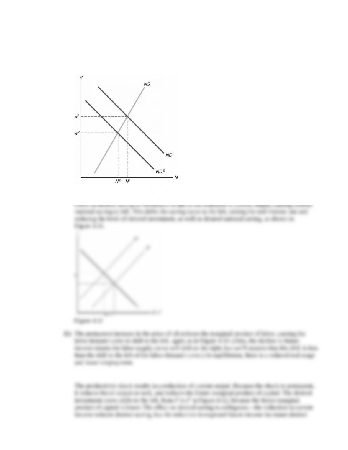
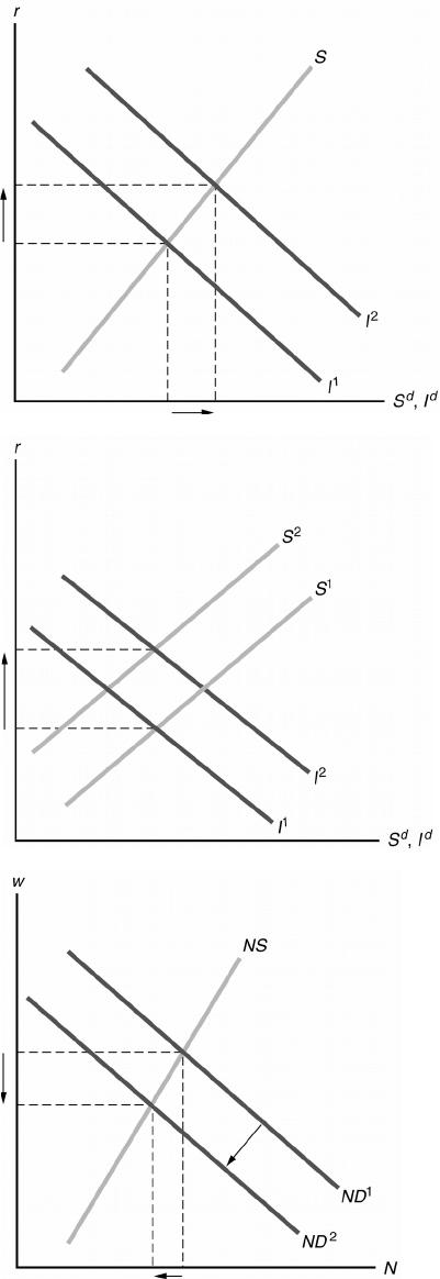
3. (a) The temporary increase in the price of oil reduces the marginal product of labor, causing the labor
demand curve to shift to the left from ND1 to ND2 in Figure 4.10. At equilibrium, there is a
reduced real wage and lower employment.
Figure 4.10
The productivity shock results in a reduction of output. Because the shock is temporary, the only
Figure 4.11
(b) The permanent increase in the price of oil reduces the marginal product of labor, causing the
labor demand curve to shift to the left, again as in Figure 4.10. (Also, the decline in future
income means the labor-supply curve will shift to the right; but we’ll assume that this shift is less
than the shift to the left of the labor–demand curve.) At equilibrium, there is a reduced real wage
and lower employment.
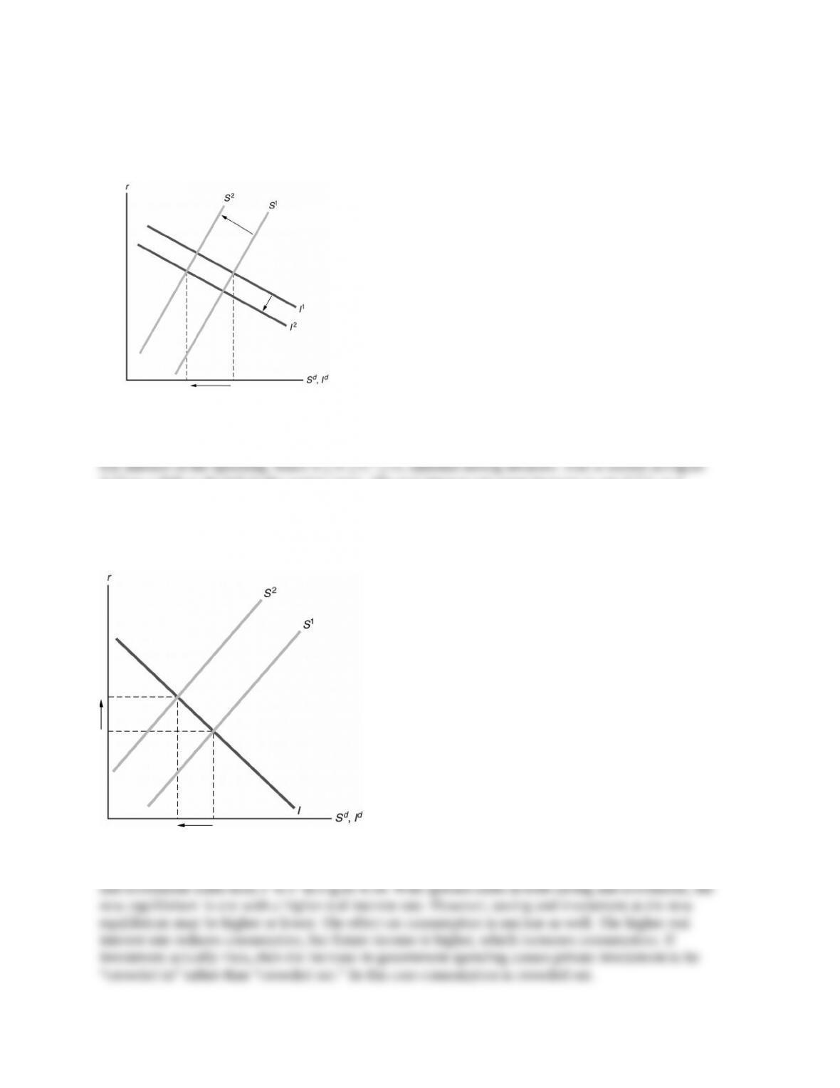
The productivity shock results in a reduction of current output. Because the shock is permanent,
it reduces future output as well, and reduces the future marginal product of capital. The desired
investment curve shifts to the left, from I1 to I2 in Figure 4.12, because the future marginal
product of capital is lower. The effect on desired saving is ambiguous—the reduction in current
income reduces desired saving, but the reduction in expected future income increases desired
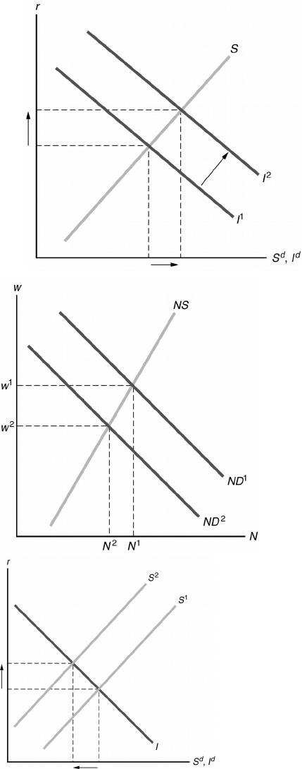
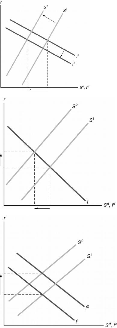
4. A temporary increase in government spending reduces national saving. Whether the spending is
financed by current taxes or by borrowing (and raising future taxes), consumption falls, but not by the
4.13 as a shift to the left in the saving curve. The real interest rate must increase to get S I, so I
declines as well. It makes no difference whether the temporary increase in spending is funded by
taxes or by borrowing.
Figure 4.13
In the case of infrastructure spending, MPKf rises, so investment increases. Saving shifts from S1 to S2
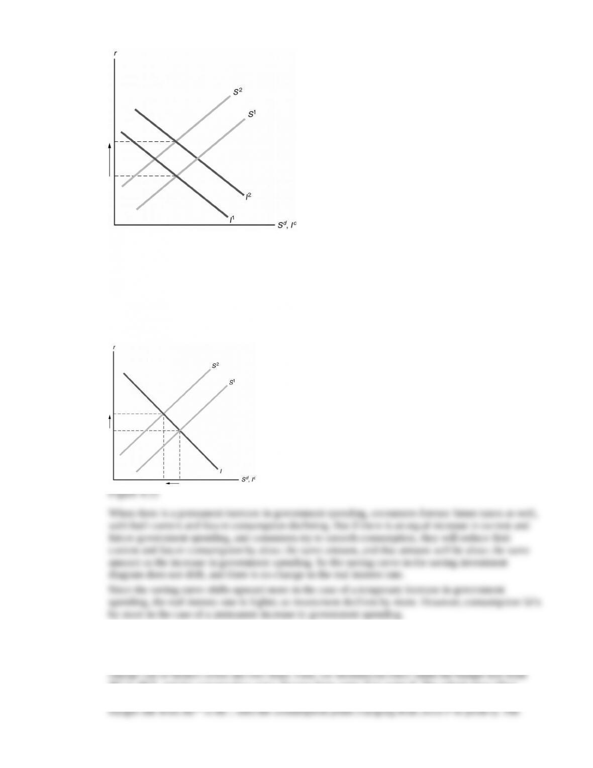
5. When there is a temporary increase in government spending, consumers foresee future taxes. As a
result, consumption declines, both currently and in the future. Thus current consumption does not fall
by as much as the increase in G, so national saving (Sd Y Cd G) declines at the initial real
interest rate, and the saving curve shifts to the left from S1 to S2, as shown in Figure 4.15. Thus the
real interest rate increases and consumption and investment both fall.
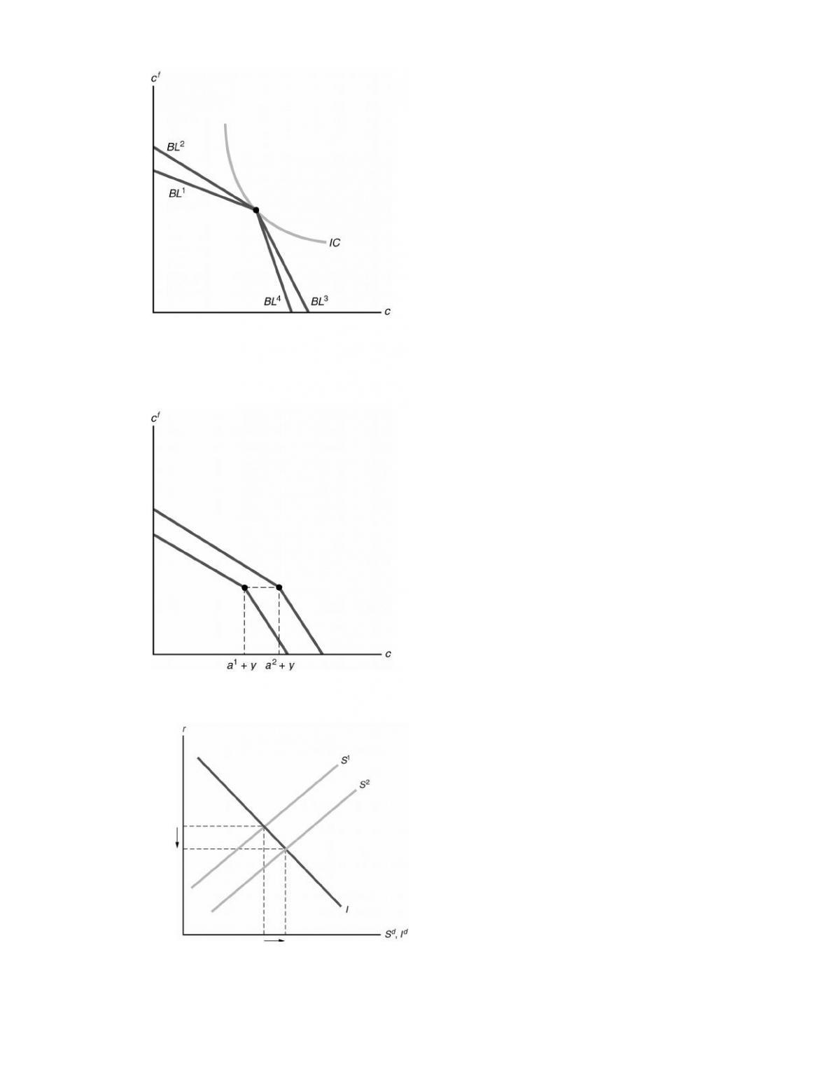
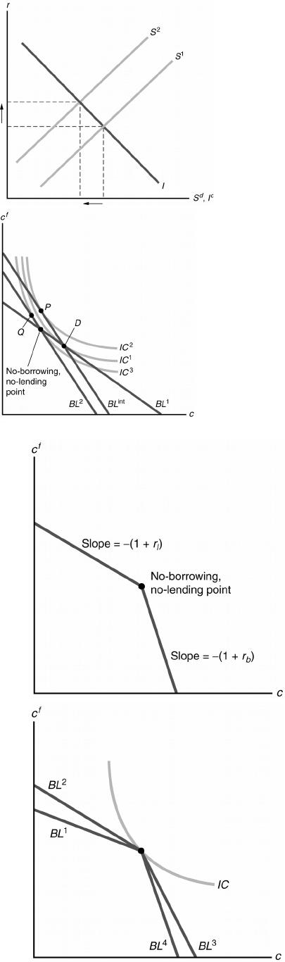
6. See Figure 4.16. The consumer is originally on budget line BL1, with consumption at point D. An
increase in the real interest rate shifts the budget line to BL2, with consumption at point Q. The
BL1 to BLint, and the consumption point changes from point D to point P. The substitution effect
results in higher future consumption and lower current consumption. The income effect shifts the
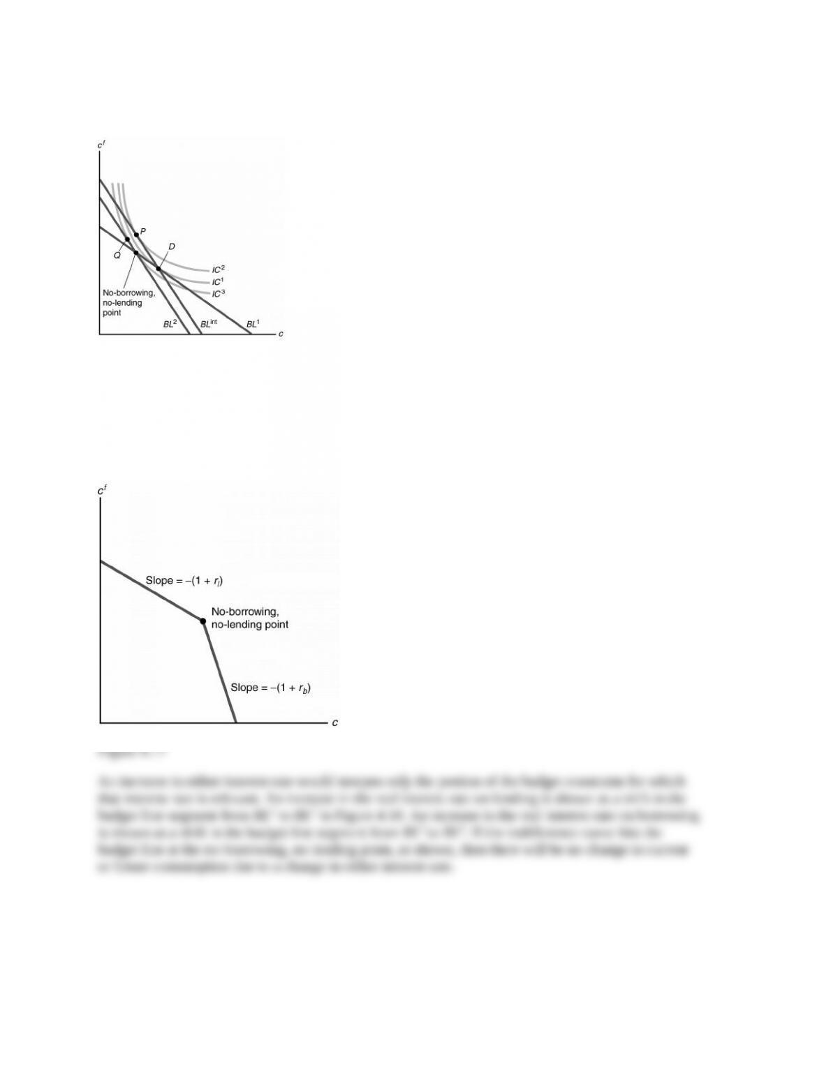
7. The difference in interest rates between borrowing and lending means there is a kink in the budget
constraint at the no-lending, no-borrowing point, as shown in Figure 4.17. Borrowing is zero when
c y a. If current consumption is less than y a, the person is a saver (lender), and the budget line
has slope (1 rl). If current consumption is greater than y a, the person is a borrower, and faces
a steeper budget constraint with slope (1 rb), because the interest rate is higher.
4. A temporary increase in government spending reduces national saving. Whether the spending is
financed by current taxes or by borrowing (and raising future taxes), consumption falls, but not by the
4.13 as a shift to the left in the saving curve. The real interest rate must increase to get S I, so I
declines as well. It makes no difference whether the temporary increase in spending is funded by
taxes or by borrowing.
Figure 4.13
In the case of infrastructure spending, MPKf rises, so investment increases. Saving shifts from S1 to S2
5. When there is a temporary increase in government spending, consumers foresee future taxes. As a
result, consumption declines, both currently and in the future. Thus current consumption does not fall
by as much as the increase in G, so national saving (Sd Y Cd G) declines at the initial real
interest rate, and the saving curve shifts to the left from S1 to S2, as shown in Figure 4.15. Thus the
real interest rate increases and consumption and investment both fall.
6. See Figure 4.16. The consumer is originally on budget line BL1, with consumption at point D. An
increase in the real interest rate shifts the budget line to BL2, with consumption at point Q. The
BL1 to BLint, and the consumption point changes from point D to point P. The substitution effect
results in higher future consumption and lower current consumption. The income effect shifts the
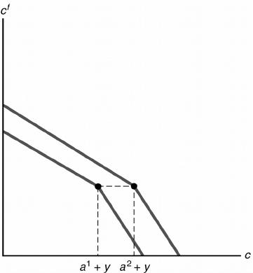
7. The difference in interest rates between borrowing and lending means there is a kink in the budget
constraint at the no-lending, no-borrowing point, as shown in Figure 4.17. Borrowing is zero when
c y a. If current consumption is less than y a, the person is a saver (lender), and the budget line
has slope (1 rl). If current consumption is greater than y a, the person is a borrower, and faces
a steeper budget constraint with slope (1 rb), because the interest rate is higher.