
1. Desired consumption: consumption amount desired by households
1. A person can consume less than current income (saving is positive)

2. A person can consume more than current income (saving is negative)
3. Trade-off between current consumption and future consumption
a. The price of 1 unit of current consumption is 1 r units of future consumption, where
1. Increase in current income: both consumption and saving increase (vice versa for decrease
in current income)
2. Marginal propensity to consume (MPC) fraction of additional current income consumed
in current period; between 0 and 1
3. Aggregate level: When current income (Y) rises, Cd rises, but not by as much as Y,
so Sd rises
Theoretical Application
The classic discussions of consumption are the permanent-income hypothesis of Milton
1. Higher expected future income leads to more consumption today, so saving falls
2. Application: consumer sentiment and forecasts of consumer spending
a. Do consumer sentiment indexes help economists forecast consumer spending?
1. Increase in wealth raises current consumption, so lowers current saving
F. Effect of changes in real interest rate
1. Increased real interest rate has two opposing effects
a. Substitution effect: Positive effect on saving, since rate of return is higher; greater reward
for saving elicits more saving
b. Income effect
(1) For a saver: Negative effect on saving, since it takes less saving to obtain a given

2. Taxes and the real return to saving
a. Expected after-tax real interest rate:
ra–t (1 t)i e(4.2)
b. Simple examples: i 5%, e 2%; if t 30%, ra–t 1.5%; if t 20%, ra–t 2%
Data Application
3. In touch with data and research: interest rates
a. Discusses different interest rates, default risk, term structure (yield curve), and tax status
1. Affects desired consumption through changes in current and expected future income
2. Directly affects desired national saving, Sd Y Cd G
3. Government purchases (temporary increase)
a. Higher G financed by higher current taxes reduces after-tax income, lowering desired
consumption
b. Even true if financed by higher future taxes, if people realize how future incomes are affected
c. Since Cd declines less than G rises, national saving (Sd Y Cd G) declines

4. Taxes
a. Lump-sum tax cut today, financed by higher future taxes
b. Decline in future income may offset increase in current income; desired consumption
could rise or fall
c. Ricardian equivalence proposition
1. The government provided tax rebates in the recessions of 2001 and 2007-2009, hoping to
stimulate the economy
2. Research by Shapiro and Slemrod suggests that consumers did not increase spending much
in 2001, when the government provided a similar tax rebate
3. New research by Agarwal, Liu, and Souleles finds that even though consumers originally
saved much of the tax rebate, later they increased spending and increased their credit-card debt
4. The new research comes from credit-card payments, purchases, and debt over time
5. People getting the tax rebates initially made additional payments on their credit cards,
paying down their balances; but after nine months they had increased their purchases and
6. Younger people, who were more likely to face binding borrowing constraints, increased
their purchases on credit cards the most of any group in response to the tax rebate
7. People with high credit limits also tended to pay off more of their balances and spent less, as
they were less likely to face binding borrowing constraints and behaved more in the manner
8. New evidence on the tax rebates in 2008 and 2009 was provided in a research paper by
Parker et al., who found that consumers spent 50%-90% of the tax rebates, which is
1. Investment fluctuates sharply over the business cycle, so we need to understand investment
to understand the business cycle
2. Investment plays a crucial role in economic growth
B. The desired capital stock
1. Desired capital stock is the amount of capital that allows firms to earn the largest expected profit
2. Desired capital stock depends on costs and benefits of additional capital
3. Since investment becomes capital stock with a lag, the benefit of investment is the future
marginal product of capital (MPKf)
4. The user cost of capital
a. Example of Kyle’s Bakery: cost of capital, depreciation rate, and expected real interest rate
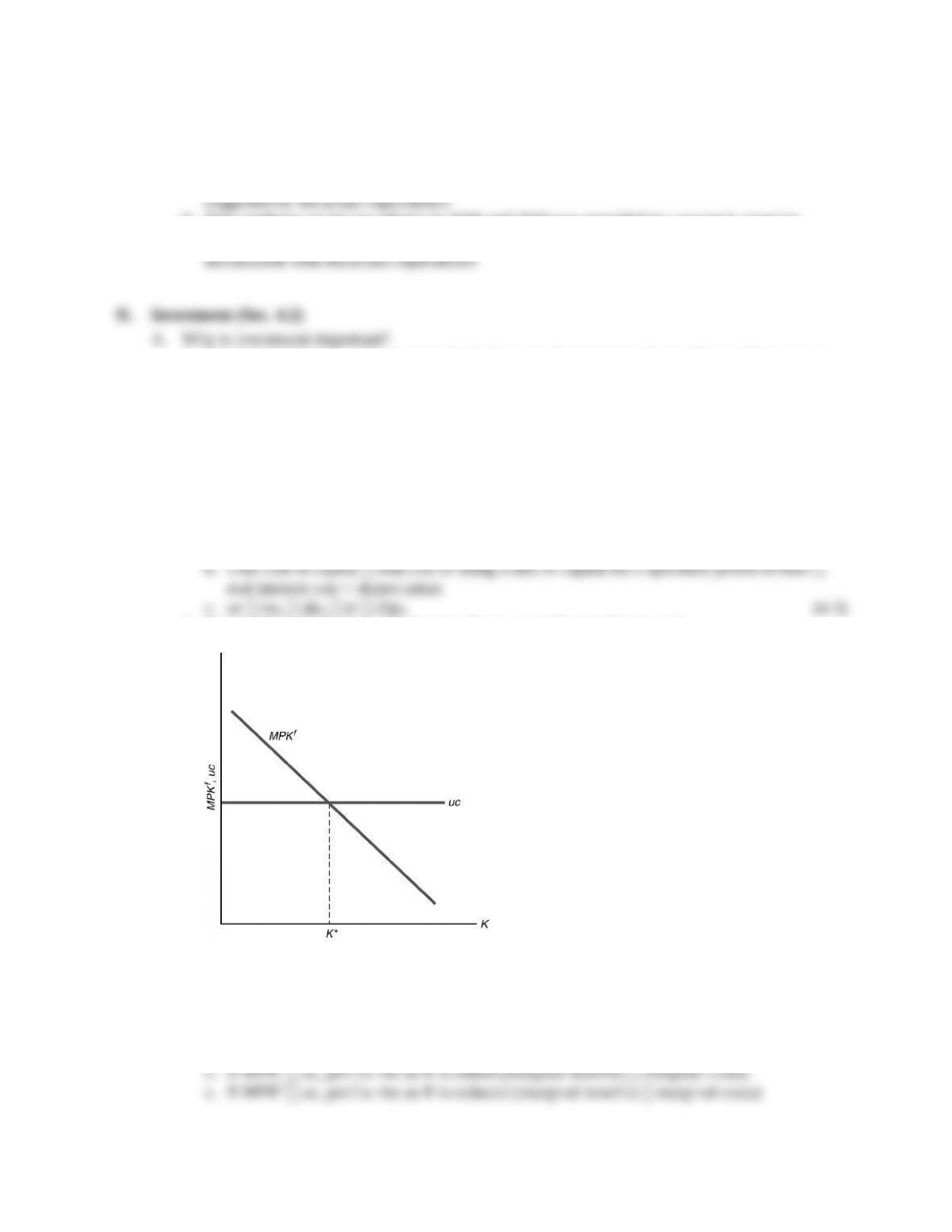
5. Determining the desired capital stock (Figure 4.1; like text Figure 4.3)
Figure 4.1
a. Desired capital stock is the level of capital stock at which MPKf uc
b. MPKf falls as K rises due to diminishing marginal productivity
c. uc doesn’t vary with K, so is a horizontal line

1. Factors that shift the MPKf curve or change the user cost of capital cause the desired capital
stock to change
2. These factors are changes in the real interest rate, depreciation rate, price of capital, or
technological changes that affect the MPKf (text Figure 4.4 shows effect of change in uc)
3. Taxes and the desired capital stock
a. With taxes, the return to capital is only (1 )MPKf
b. A firm chooses its desired capital stock so that the return equals the user cost, so
(1 )MPKf uc, which means:
MPKf uc/(1 ) (r d)pK/(1 ) (4.4)
1. The capital stock changes from two opposing channels
a. New capital increases the capital stock; this is gross investment
2. Rewriting (4.5) gives It Kt+1 Kt dKt
a. If firms can change their capital stocks in one period, then the desired capital stock
3. Lags and investment
a. Some capital can be constructed easily, but other capital may take years to put in place
Theoretical Application
Acknowledging that it may take time to get capital in place may be crucial to modeling the
1. Firms change investment in the same direction as the stock market: Tobin’s q theory of
investment
2. If market value replacement cost, then firm should invest more
3. Tobin’s q capital’s market value divided by its replacement cost
a. If q 1, don’t invest
4. Stock price times number of shares equals firm’s market value, which equals value
of firm’s capital
5. Data show general tendency of investment to rise when stock market rises; but relationship
isn’t strong because many other things change at same time (text Fig. 4.7)
6. This theory is similar to text discussion
a. Higher MPKf increases future earnings of firm, so V rises

1. Marginal product of capital and user cost also apply, as with equipment and structures
Numerical Problem 3 applies the user-cost concept to the purchase or rental of a home.
1. Y Cd Id G(4.7)
goods market equilibrium condition
2. Differs from income-expenditure identity, as goods market equilibrium condition need not
hold; undesired goods may be produced, so goods market won’t be in equilibrium
3. Alternative representation: since
Sd Y Cd G,
1. Plot Sd vs. Id (Figure 4.2; Key Diagram 3; like text Figure 4.8)
Figure 4.2
2. Equilibrium where Sd Id
3. How to reach equilibrium? Adjustment of r
4. Shifts of the saving curve
a. Saving curve shifts right due to a rise in current output, a fall in expected future output,
a fall in wealth, a fall in government purchases, a rise in taxes (unless Ricardian
equivalence holds, in which case tax changes have no effect)
b. Example: Temporary increase in government purchases shifts S left
5. Shifts of the investment curve
a. Investment curve shifts right due to a fall in the effective tax rate or a rise in expected
1. Sharp changes in stock prices affect consumption spending (a wealth effect) and capital
investment (via Tobin’s q), seen in text Figure 4.11
2. Consumption and the 1987 crash
a. When the stock market crashed in 1987, wealth declined by about $1 trillion
b. Consumption fell somewhat less than might be expected, and it wasn’t enough
to cause a recession
3. Consumption and the rise in stock market wealth in the 1990s
a. Stock prices more than tripled in real terms
4. Consumption and the decline in stock prices in the early 2000s
a. In the early 2000s, wealth in stocks declined by about $5 trillion
5. Investment and the declines in the stock market in the 2000s
a. Investment and Tobin’s q were correlated in 2000 and 2008, when the stock market fell
6. The financial crisis of 2008
a. Stock prices plunged in fall 2008 and early 2009, and home prices fell sharply as well,
2. A person can consume more than current income (saving is negative)
3. Trade-off between current consumption and future consumption
a. The price of 1 unit of current consumption is 1 r units of future consumption, where
1. Increase in current income: both consumption and saving increase (vice versa for decrease
in current income)
2. Marginal propensity to consume (MPC) fraction of additional current income consumed
in current period; between 0 and 1
3. Aggregate level: When current income (Y) rises, Cd rises, but not by as much as Y,
so Sd rises
Theoretical Application
The classic discussions of consumption are the permanent-income hypothesis of Milton
1. Higher expected future income leads to more consumption today, so saving falls
2. Application: consumer sentiment and forecasts of consumer spending
a. Do consumer sentiment indexes help economists forecast consumer spending?
1. Increase in wealth raises current consumption, so lowers current saving
F. Effect of changes in real interest rate
1. Increased real interest rate has two opposing effects
a. Substitution effect: Positive effect on saving, since rate of return is higher; greater reward
for saving elicits more saving
b. Income effect
(1) For a saver: Negative effect on saving, since it takes less saving to obtain a given
2. Taxes and the real return to saving
a. Expected after-tax real interest rate:
ra–t (1 t)i e(4.2)
b. Simple examples: i 5%, e 2%; if t 30%, ra–t 1.5%; if t 20%, ra–t 2%
Data Application
3. In touch with data and research: interest rates
a. Discusses different interest rates, default risk, term structure (yield curve), and tax status
1. Affects desired consumption through changes in current and expected future income
2. Directly affects desired national saving, Sd Y Cd G
3. Government purchases (temporary increase)
a. Higher G financed by higher current taxes reduces after-tax income, lowering desired
consumption
b. Even true if financed by higher future taxes, if people realize how future incomes are affected
c. Since Cd declines less than G rises, national saving (Sd Y Cd G) declines
4. Taxes
a. Lump-sum tax cut today, financed by higher future taxes
b. Decline in future income may offset increase in current income; desired consumption
could rise or fall
c. Ricardian equivalence proposition
1. The government provided tax rebates in the recessions of 2001 and 2007-2009, hoping to
stimulate the economy
2. Research by Shapiro and Slemrod suggests that consumers did not increase spending much
in 2001, when the government provided a similar tax rebate
3. New research by Agarwal, Liu, and Souleles finds that even though consumers originally
saved much of the tax rebate, later they increased spending and increased their credit-card debt
4. The new research comes from credit-card payments, purchases, and debt over time
5. People getting the tax rebates initially made additional payments on their credit cards,
paying down their balances; but after nine months they had increased their purchases and
6. Younger people, who were more likely to face binding borrowing constraints, increased
their purchases on credit cards the most of any group in response to the tax rebate
7. People with high credit limits also tended to pay off more of their balances and spent less, as
they were less likely to face binding borrowing constraints and behaved more in the manner
8. New evidence on the tax rebates in 2008 and 2009 was provided in a research paper by
Parker et al., who found that consumers spent 50%-90% of the tax rebates, which is
1. Investment fluctuates sharply over the business cycle, so we need to understand investment
to understand the business cycle
2. Investment plays a crucial role in economic growth
B. The desired capital stock
1. Desired capital stock is the amount of capital that allows firms to earn the largest expected profit
2. Desired capital stock depends on costs and benefits of additional capital
3. Since investment becomes capital stock with a lag, the benefit of investment is the future
marginal product of capital (MPKf)
4. The user cost of capital
a. Example of Kyle’s Bakery: cost of capital, depreciation rate, and expected real interest rate
5. Determining the desired capital stock (Figure 4.1; like text Figure 4.3)
Figure 4.1
a. Desired capital stock is the level of capital stock at which MPKf uc
b. MPKf falls as K rises due to diminishing marginal productivity
c. uc doesn’t vary with K, so is a horizontal line
1. Factors that shift the MPKf curve or change the user cost of capital cause the desired capital
stock to change
2. These factors are changes in the real interest rate, depreciation rate, price of capital, or
technological changes that affect the MPKf (text Figure 4.4 shows effect of change in uc)
3. Taxes and the desired capital stock
a. With taxes, the return to capital is only (1 )MPKf
b. A firm chooses its desired capital stock so that the return equals the user cost, so
(1 )MPKf uc, which means:
MPKf uc/(1 ) (r d)pK/(1 ) (4.4)
1. The capital stock changes from two opposing channels
a. New capital increases the capital stock; this is gross investment
2. Rewriting (4.5) gives It Kt+1 Kt dKt
a. If firms can change their capital stocks in one period, then the desired capital stock
3. Lags and investment
a. Some capital can be constructed easily, but other capital may take years to put in place
Theoretical Application
Acknowledging that it may take time to get capital in place may be crucial to modeling the
1. Firms change investment in the same direction as the stock market: Tobin’s q theory of
investment
2. If market value replacement cost, then firm should invest more
3. Tobin’s q capital’s market value divided by its replacement cost
a. If q 1, don’t invest
4. Stock price times number of shares equals firm’s market value, which equals value
of firm’s capital
5. Data show general tendency of investment to rise when stock market rises; but relationship
isn’t strong because many other things change at same time (text Fig. 4.7)
6. This theory is similar to text discussion
a. Higher MPKf increases future earnings of firm, so V rises
1. Marginal product of capital and user cost also apply, as with equipment and structures
Numerical Problem 3 applies the user-cost concept to the purchase or rental of a home.
1. Y Cd Id G(4.7)
goods market equilibrium condition
2. Differs from income-expenditure identity, as goods market equilibrium condition need not
hold; undesired goods may be produced, so goods market won’t be in equilibrium
3. Alternative representation: since
Sd Y Cd G,
1. Plot Sd vs. Id (Figure 4.2; Key Diagram 3; like text Figure 4.8)
Figure 4.2
2. Equilibrium where Sd Id
3. How to reach equilibrium? Adjustment of r
4. Shifts of the saving curve
a. Saving curve shifts right due to a rise in current output, a fall in expected future output,
a fall in wealth, a fall in government purchases, a rise in taxes (unless Ricardian
equivalence holds, in which case tax changes have no effect)
b. Example: Temporary increase in government purchases shifts S left
5. Shifts of the investment curve
a. Investment curve shifts right due to a fall in the effective tax rate or a rise in expected
1. Sharp changes in stock prices affect consumption spending (a wealth effect) and capital
investment (via Tobin’s q), seen in text Figure 4.11
2. Consumption and the 1987 crash
a. When the stock market crashed in 1987, wealth declined by about $1 trillion
b. Consumption fell somewhat less than might be expected, and it wasn’t enough
to cause a recession
3. Consumption and the rise in stock market wealth in the 1990s
a. Stock prices more than tripled in real terms
4. Consumption and the decline in stock prices in the early 2000s
a. In the early 2000s, wealth in stocks declined by about $5 trillion
5. Investment and the declines in the stock market in the 2000s
a. Investment and Tobin’s q were correlated in 2000 and 2008, when the stock market fell
6. The financial crisis of 2008
a. Stock prices plunged in fall 2008 and early 2009, and home prices fell sharply as well,