Figure 3.6
the 1970s and early 1980s had to do with the increased participation rates of women in the labor
force. Research on both the causes and consequences of this change occupied many economists
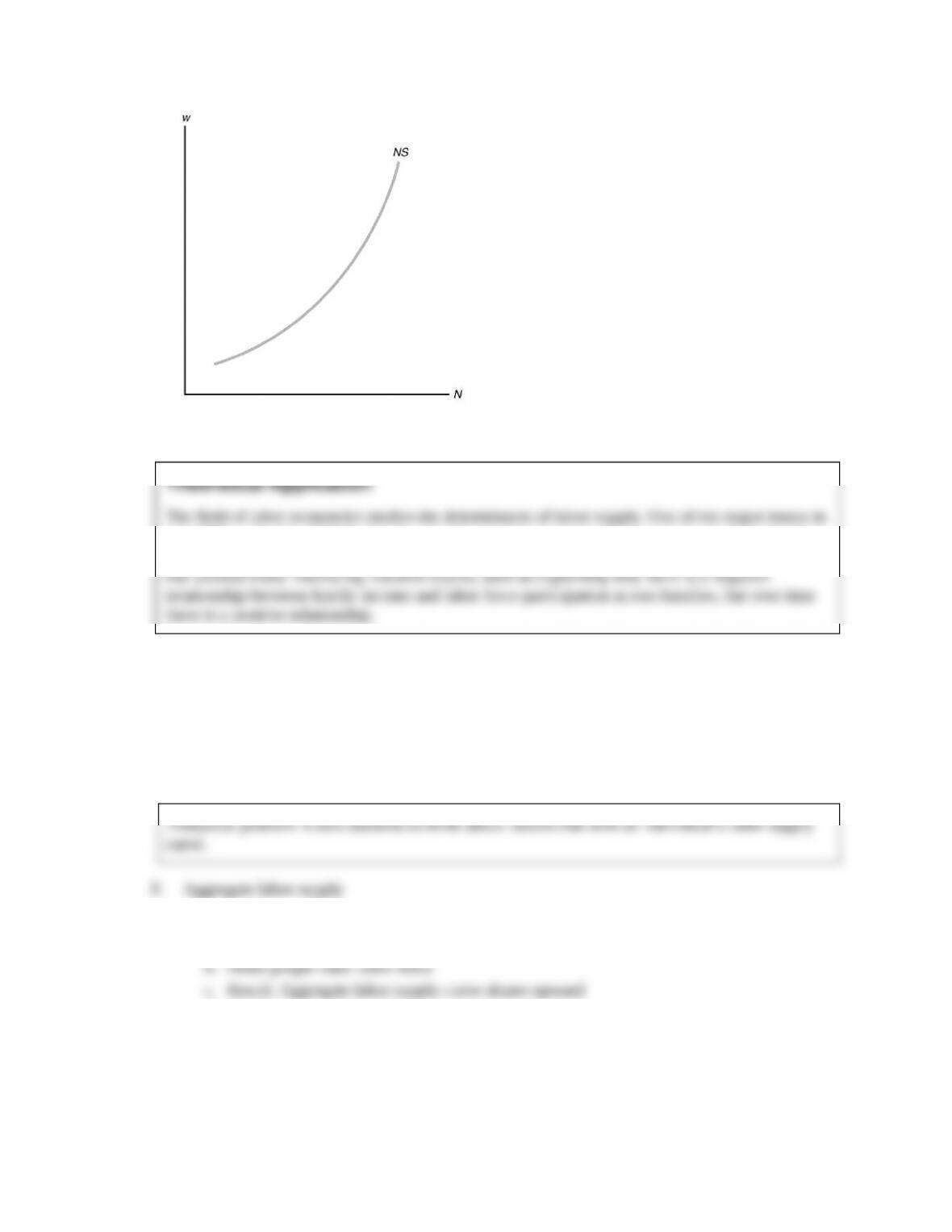
3. Labor supply curve slopes upward because higher wage encourages people to work more
E. Factors that shift the labor supply curve
1. Wealth: Higher wealth reduces labor supply (shifts labor supply curve to the left; text
Fig. 3.8)
2. Expected future real wage: Higher expected future real wage is like an increase in wealth,
so reduces labor supply (shifts labor supply curve to the left)
1. Aggregate labor supply rises when current real wage rises
a. Some people work more hours
2. Factors increasing labor supply
a. Decrease in wealth
b. Decrease in expected future real wage
c. Increase in working-age population (higher birth rate, immigration)

the 1990s, women’s LFPR growth slowed, probably due to both economics (a discouraged
worker effect) and social considerations (an increased fertility rate). These factors continued in
the 2000s, and women’s LFPR declined from about 60% in 2000 to about 58% in 2012.
IV. Labor Market Equilibrium (Sec. 3.4)
1. Classical model of the labor market—real wage adjusts quickly (later, in Chapter 11, look at
other models of labor market in which real wage does not adjust quickly)
N
N
N
w

1960s 27%
1970s 13%
1980s 5%
1990s 14%
2000s 13%
B. Full-employment output
Y
Y
Y
Y
N
3.
Y
affected by changes in
N
or production function (example: supply shock, text Fig. 3.10)
1. Sharp oil price increases in 1973–1974, 1979–1980, 2003–2008 (text Fig. 3.11)
2. Adverse supply shock—lowers labor demand, employment, the real wage, and the full-
employment level of output
3. First two cases: U.S. economy entered recessions
4. Research result: 10% increase in price of oil reduces GDP by 0.4 percentage points

V. Unemployment (Sec. 3.5)
1. Categories: employed, unemployed, not in the labor force
2. Labor Force Employed Unemployed
3. Unemployment Rate Unemployed/Labor Force
4. Table 3.4 shows current data
Data Application
The unemployment rate jumped up sharply in January 1994, not because of any true change in
the labor market, but merely because the Bureau of Labor Statistics changed the survey with
4. Participation Rate Labor Force/Adult Population
5. Employment Ratio Employed/Adult Population
Analytical Problem 6 tests students’ ability to use these different measures.
1. Flows between categories (text Fig. 3.12)
2. Discouraged workers: people who have become so discouraged by lack of success at finding
a job that they stop searching
1996.
Numerical Problems 7 and 8 are quantitative exercises using the unemployment and employment
1. Most unemployment spells are of short duration
a. Unemployment spell period of time an individual is continuously unemployed
2. Most unemployed people on a given date are experiencing unemployment spells of long
duration
3. Reconciling 1 and 2—numerical example:

a. Labor force 100; on the first day of every month, two workers become unemployed for
one month each; on the first day of every year, four workers become unemployed for
one year each
1. The mean duration of unemployment always rises in recessions but in the 2007-2009 the rise
was larger than ever before (text Fig. 3.13)
2. Four possible explanations for the increase include measurement issues, the extension of
unemployment benefits, very large job losses, and a weak economic recovery
1. Frictional unemployment
a. Search activity of firms and workers due to heterogeneity
b. Matching process takes time
Policy Application
2. Structural unemployment
a. Chronically unemployed: workers who are unemployed a large part of the time
3. The natural rate of unemployment
a.
u
natural rate of unemployment; when output and employment are at full-
employment levels
u

4. In touch with data and research: labor market data
a. BLS employment report
(1) Household survey: unemployment, employment
(2) Establishment survey: jobs
Data Application
1. Other things happen when cyclical unemployment rises: Labor force falls, hours of work per
worker decline, average productivity of labor declines
2. Result is 2% reduction in output associated with 1 percentage point increase in
unemployment rate
1. Y/Y 3 2 u(3.6)
2. Text Fig. 3.14 shows U.S. data
Data Application

In 2009, the unemployment rate increased far more than expected (or, output did not decline as
much as expected) under Okun’s law. The reason was remarkably strong growth in productivity
the 1990s, women’s LFPR growth slowed, probably due to both economics (a discouraged
worker effect) and social considerations (an increased fertility rate). These factors continued in
the 2000s, and women’s LFPR declined from about 60% in 2000 to about 58% in 2012.
IV. Labor Market Equilibrium (Sec. 3.4)
1. Classical model of the labor market—real wage adjusts quickly (later, in Chapter 11, look at
other models of labor market in which real wage does not adjust quickly)
N
w
1960s 27%
1970s 13%
1980s 5%
1990s 14%
2000s 13%
B. Full-employment output
N
3.
Y
affected by changes in
N
or production function (example: supply shock, text Fig. 3.10)
1. Sharp oil price increases in 1973–1974, 1979–1980, 2003–2008 (text Fig. 3.11)
2. Adverse supply shock—lowers labor demand, employment, the real wage, and the full-
employment level of output
3. First two cases: U.S. economy entered recessions
4. Research result: 10% increase in price of oil reduces GDP by 0.4 percentage points
V. Unemployment (Sec. 3.5)
1. Categories: employed, unemployed, not in the labor force
2. Labor Force Employed Unemployed
3. Unemployment Rate Unemployed/Labor Force
4. Table 3.4 shows current data
Data Application
The unemployment rate jumped up sharply in January 1994, not because of any true change in
the labor market, but merely because the Bureau of Labor Statistics changed the survey with
4. Participation Rate Labor Force/Adult Population
5. Employment Ratio Employed/Adult Population
Analytical Problem 6 tests students’ ability to use these different measures.
1. Flows between categories (text Fig. 3.12)
2. Discouraged workers: people who have become so discouraged by lack of success at finding
a job that they stop searching
1996.
Numerical Problems 7 and 8 are quantitative exercises using the unemployment and employment
1. Most unemployment spells are of short duration
a. Unemployment spell period of time an individual is continuously unemployed
2. Most unemployed people on a given date are experiencing unemployment spells of long
duration
3. Reconciling 1 and 2—numerical example:
a. Labor force 100; on the first day of every month, two workers become unemployed for
one month each; on the first day of every year, four workers become unemployed for
one year each
1. The mean duration of unemployment always rises in recessions but in the 2007-2009 the rise
was larger than ever before (text Fig. 3.13)
2. Four possible explanations for the increase include measurement issues, the extension of
unemployment benefits, very large job losses, and a weak economic recovery
1. Frictional unemployment
a. Search activity of firms and workers due to heterogeneity
b. Matching process takes time
Policy Application
2. Structural unemployment
a. Chronically unemployed: workers who are unemployed a large part of the time
3. The natural rate of unemployment
a.
u
natural rate of unemployment; when output and employment are at full-
employment levels
u
4. In touch with data and research: labor market data
a. BLS employment report
(1) Household survey: unemployment, employment
(2) Establishment survey: jobs
Data Application
1. Other things happen when cyclical unemployment rises: Labor force falls, hours of work per
worker decline, average productivity of labor declines
2. Result is 2% reduction in output associated with 1 percentage point increase in
unemployment rate
1. Y/Y 3 2 u(3.6)
2. Text Fig. 3.14 shows U.S. data
Data Application
In 2009, the unemployment rate increased far more than expected (or, output did not decline as
much as expected) under Okun’s law. The reason was remarkably strong growth in productivity