
Chapter 3
1. Three markets
a. Labor market (this chapter)
b. Goods market (Ch. 4)
c. Asset market (Ch. 7)
II. Goals of Chapter 3
B. A new application “Unemployment Duration and the 2007-2009 Recession” was added
Teaching Notes
1. Capital (K)
2. Labor (N)
3. Others (raw materials, land, energy)
4. Productivity of factors depends on technology and management
B. The production function
1. Y AF(K, N) (3.1)
2. Parameter A is “total factor productivity” (the effectiveness with which capital and labor
are used)
1. Cobb-Douglas production function works well for U.S. economy:
Y A K 0.3 N 0.7 (3.2)
2. Data for U.S. economy—text Table 3.1
Numerical Problem 1 gives students practice working with a production function.
3. Productivity growth calculated using production function
a. Productivity moves sharply from year to year
Data Application
An example of the sharp movements in productivity that are possible can be seen by comparing
data on productivity for 2003 to data for 2004. Employment grew about the same amount in
the 2000s
Policy Application
1. Two main properties of production functions
a. Slopes upward: more of any input produces more output
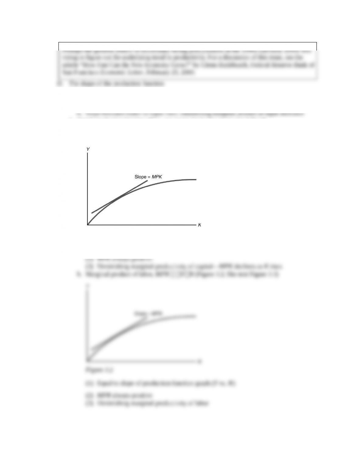
2. Graph production function (Y vs. one input; hold other input and A fixed)
a. Marginal product of capital, MPK Y/K (Figure 3.1; Key Diagram 1; like text
Figure 3.2)
Figure 3.1
(1) Equal to slope of production function graph (Y vs. K)
1. Supply shock productivity shock a change in an economy’s production function
2. Supply shocks affect the amount of output that can be produced for a given amount of inputs
3. Shocks may be positive (increasing output) or negative (decreasing output)
4. Examples: weather, inventions and innovations, government regulations, oil prices
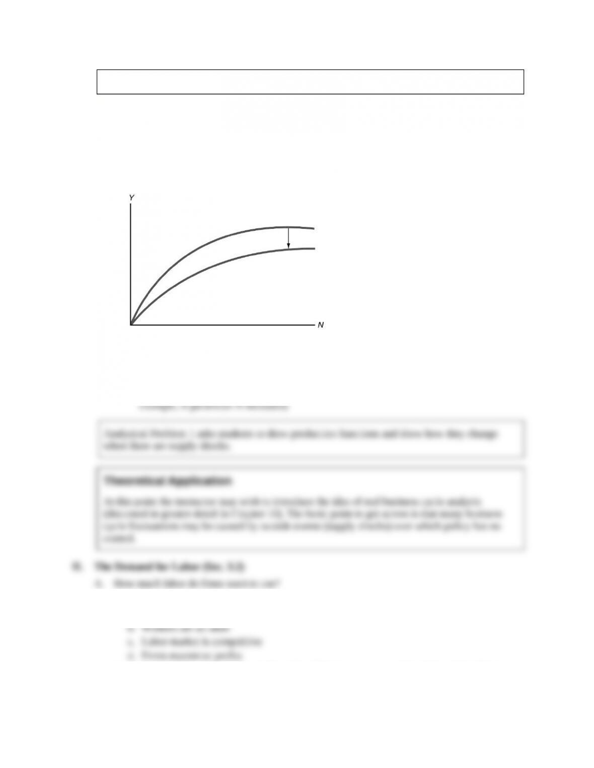
5. Supply shocks shift graph of production function (Figure 3.3; like text Figure 3.4)
Figure 3.3
a. Negative (adverse) shock: Usually slope of production function decreases at each level of
input (for example, if shock causes parameter A to decline)
b. Positive shock: Usually slope of production function increases at each level of output (for
1. Assumptions
a. Hold capital stock fixed—short-run analysis
2. Analysis at the margin: costs and benefits of hiring one extra worker (Figure 3.4; like text
Figure 3.5)
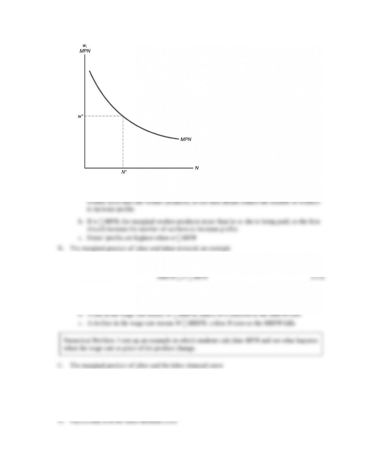
Figure 3.4
a. If real wage (w) marginal product of labor (MPN), the firm is paying the marginal
1. Example: The Clip Joint—setting the nominal wage equal to the marginal revenue product
of labor
2. W MRPN is the same condition as w MPN, since W P w and MRPN P MPN
3. A change in the wage
a. Begin at equilibrium where W MRPN
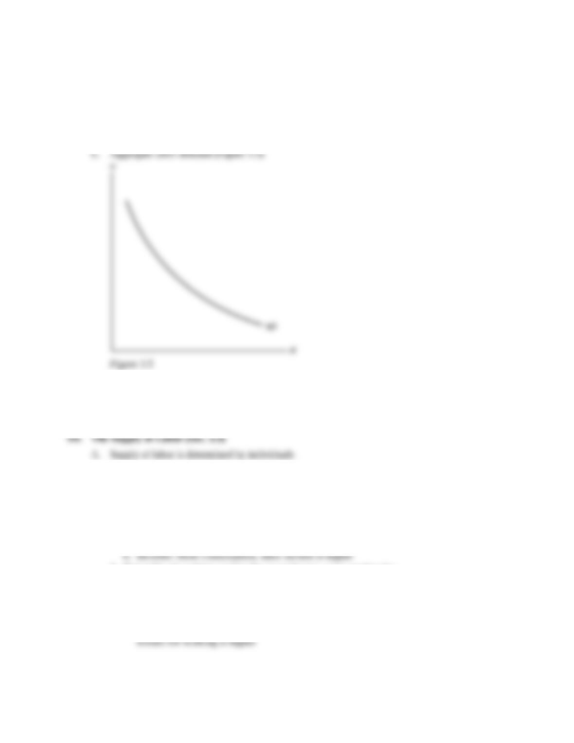
1. Labor demand curve shows relationship between the real wage rate and the quantity of labor
demanded
2. It is the same as the MPN curve, since w MPN at equilibrium
3. So the labor demand curve is downward sloping; firms want to hire less labor, the higher the
real wage
1. Note: A change in the wage causes a movement along the labor demand curve, not a shift of
the curve
2. Supply shocks: Beneficial supply shock raises MPN, so shifts labor demand curve to the
right; opposite for adverse supply shock
3. Size of capital stock: Higher capital stock raises MPN, so shifts labor demand curve to the
right; opposite for lower capital stock
1. Aggregate labor demand is the sum of all firms’ labor demand
2. Same factors (supply shocks, size of capital stock) that shift firms’ labor demand cause
shifts in aggregate labor demand
1. Aggregate supply of labor is sum of individuals’ labor supply
2. Labor supply of individuals depends on labor-leisure choice
B. The income-leisure trade-off
1. Utility depends on consumption and leisure
2. Need to compare costs and benefits of working another day
a. Costs: Loss of leisure time
3. If benefits of working another day exceed costs, work another day
4. Keep working additional days until benefits equal costs
C. Real wages and labor supply
1. An increase in the real wage has offsetting income and substitution effects
a. Substitution effect of a higher real wage: Higher real wage encourages work, since the

2. A pure substitution effect: a one-day rise in the real wage
a. A temporary real wage increase has just a pure substitution effect, since the effect on
3. A pure income effect: winning the lottery
a. Winning the lottery doesn’t have a substitution effect, because it doesn’t affect the
4. The substitution effect and the income effect together: a long-term increase in the real wage
a. The reward to working is greater: a substitution effect toward more work
5. Empirical evidence on real wages and labor supply
a. Overall result: Labor supply increases with a temporary rise in the real wage
b. Labor supply falls with a permanent increase in the real wage
Theoretical Application
1. Increase in the current real wage should raise quantity of labor supplied
2. Labor supply curve relates quantity of labor supplied to real wage
1. Capital (K)
2. Labor (N)
3. Others (raw materials, land, energy)
4. Productivity of factors depends on technology and management
B. The production function
1. Y AF(K, N) (3.1)
2. Parameter A is “total factor productivity” (the effectiveness with which capital and labor
are used)
1. Cobb-Douglas production function works well for U.S. economy:
Y A K 0.3 N 0.7 (3.2)
2. Data for U.S. economy—text Table 3.1
Numerical Problem 1 gives students practice working with a production function.
3. Productivity growth calculated using production function
a. Productivity moves sharply from year to year
Data Application
An example of the sharp movements in productivity that are possible can be seen by comparing
data on productivity for 2003 to data for 2004. Employment grew about the same amount in
the 2000s
Policy Application
1. Two main properties of production functions
a. Slopes upward: more of any input produces more output
2. Graph production function (Y vs. one input; hold other input and A fixed)
a. Marginal product of capital, MPK Y/K (Figure 3.1; Key Diagram 1; like text
Figure 3.2)
Figure 3.1
(1) Equal to slope of production function graph (Y vs. K)
1. Supply shock productivity shock a change in an economy’s production function
2. Supply shocks affect the amount of output that can be produced for a given amount of inputs
3. Shocks may be positive (increasing output) or negative (decreasing output)
4. Examples: weather, inventions and innovations, government regulations, oil prices
5. Supply shocks shift graph of production function (Figure 3.3; like text Figure 3.4)
Figure 3.3
a. Negative (adverse) shock: Usually slope of production function decreases at each level of
input (for example, if shock causes parameter A to decline)
b. Positive shock: Usually slope of production function increases at each level of output (for
1. Assumptions
a. Hold capital stock fixed—short-run analysis
2. Analysis at the margin: costs and benefits of hiring one extra worker (Figure 3.4; like text
Figure 3.5)
Figure 3.4
a. If real wage (w) marginal product of labor (MPN), the firm is paying the marginal
1. Example: The Clip Joint—setting the nominal wage equal to the marginal revenue product
of labor
2. W MRPN is the same condition as w MPN, since W P w and MRPN P MPN
3. A change in the wage
a. Begin at equilibrium where W MRPN
1. Labor demand curve shows relationship between the real wage rate and the quantity of labor
demanded
2. It is the same as the MPN curve, since w MPN at equilibrium
3. So the labor demand curve is downward sloping; firms want to hire less labor, the higher the
real wage
1. Note: A change in the wage causes a movement along the labor demand curve, not a shift of
the curve
2. Supply shocks: Beneficial supply shock raises MPN, so shifts labor demand curve to the
right; opposite for adverse supply shock
3. Size of capital stock: Higher capital stock raises MPN, so shifts labor demand curve to the
right; opposite for lower capital stock
1. Aggregate labor demand is the sum of all firms’ labor demand
2. Same factors (supply shocks, size of capital stock) that shift firms’ labor demand cause
shifts in aggregate labor demand
1. Aggregate supply of labor is sum of individuals’ labor supply
2. Labor supply of individuals depends on labor-leisure choice
B. The income-leisure trade-off
1. Utility depends on consumption and leisure
2. Need to compare costs and benefits of working another day
a. Costs: Loss of leisure time
3. If benefits of working another day exceed costs, work another day
4. Keep working additional days until benefits equal costs
C. Real wages and labor supply
1. An increase in the real wage has offsetting income and substitution effects
a. Substitution effect of a higher real wage: Higher real wage encourages work, since the
2. A pure substitution effect: a one-day rise in the real wage
a. A temporary real wage increase has just a pure substitution effect, since the effect on
3. A pure income effect: winning the lottery
a. Winning the lottery doesn’t have a substitution effect, because it doesn’t affect the
4. The substitution effect and the income effect together: a long-term increase in the real wage
a. The reward to working is greater: a substitution effect toward more work
5. Empirical evidence on real wages and labor supply
a. Overall result: Labor supply increases with a temporary rise in the real wage
b. Labor supply falls with a permanent increase in the real wage
Theoretical Application
1. Increase in the current real wage should raise quantity of labor supplied
2. Labor supply curve relates quantity of labor supplied to real wage