Additional Issues for Classroom Discussion
1. What Other Relationships Are There Between Currencies?
In financial markets, there are many relationships between the returns on different assets. In international
financial markets, these relationships depend a lot on the exchange rate. Ask your students how they
would determine how much money to invest in foreign countries. What are the returns to such investment,
translated into U.S. dollars? What risks are there? What happens to the value of your investment when the
2% (4% euro return minus 2% depreciation). The process described here is known as uncovered interest-rate
parity. It’s uncovered because it’s risky. Another process, covered interest parity, involves trades using
2. How Predictable Are Exchange Rates?
Economists’ theories of exchange rates are very well developed, especially after hundreds of years of
experience. How precisely do you think financial market participants, such as currency traders, can
forecast exchange rates?
It turns out that despite all our economic theories and extensive empirical work, forecasts of exchange
least, short-term exchange rate forecasting is far more an art than a science.
1. The nominal exchange rate is the rate at which two currencies can be exchanged for each other in the
market. The real exchange rate is the price of domestic goods relative to foreign goods. Changes in
2. The two major types of exchange-rate systems are fixed exchange rates and flexible exchange rates.
In a fixed-exchange-rate system, exchange rates are set at officially determined levels. In a flexible-
3. Purchasing power parity, PPP, is the idea that similar foreign and domestic goods, or baskets of
goods, should have the same price when priced in terms of the same currency. Purchasing power
4. The J curve shows the response of net exports to a real depreciation. At first the real depreciation
reduces net exports, as the decline in the real exchange rate means that a country pays more for its
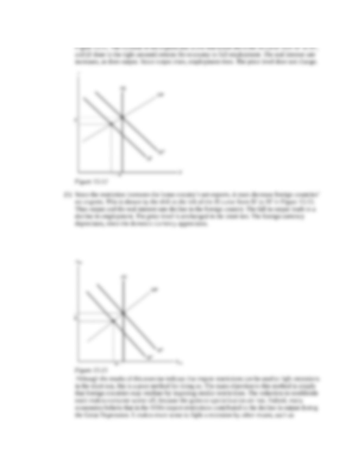
5. An increase in domestic income leads people to buy more goods, including imported goods, so net
exports decline. An increase in foreign income leads foreigners to buy more goods, including goods
6. Foreigners demand dollars in the foreign exchange market to be able to buy U.S. goods and services
(U.S. exports) and U.S. real and financial assets (U.S. capital inflows). Americans supply dollars to
the foreign exchange market to be able to buy foreign goods and services (U.S. imports) and real and
financial assets in foreign countries (U.S. capital outflows). The demand for dollars increases if the
7. The IS–LM model for the open economy differs from the closed-economy IS–LM model in that
international influences may shift the IS curve. Factors that raise a country’s net exports, given
8. Expansionary fiscal policy increases output and the real interest rate in the short run (using a
Keynesian model), both of which lead to a reduction of net exports. Expansionary monetary policy
9. In the short run, expansionary monetary policy increases output (using a Keynesian model), which
decreases net exports, leading to an increased supply of the domestic currency in the foreign
exchange market, causing it to depreciate. Expansionary monetary policy also reduces the real
interest rate, causing reduced demand for domestic assets, again causing the currency to depreciate.
10. The fundamental value of a currency is the value of the exchange rate that would be determined by
free-market forces of demand and supply without government intervention. When the official
11.A country is limited in changing its money supply under a fixed-exchange-rate system, because
only one level of the money supply is consistent with the official exchange rate being equal to its
12. Flexible exchange rates have the advantage of allowing a country to use expansionary monetary
policy to combat recessions, but currency values fluctuate substantially, introducing uncertainty
into international transactions. Fixed exchange rates avoid this problem, but a country may have to
give up the independent use of monetary policy. This latter factor is a disadvantage when it comes
1. The price level in the West is PW 5 guilders per ordinary soap bar. The price level in the East is
PE 100 florins per deluxe soap bar. The real exchange rate is 2 ordinary soap bars per deluxe
soap bar.
(a) Use Eq. (13.6) to get enom ePFOR /P 2 ordinary soap bars per deluxe soap bar 5 guilders per
2. (a) Japan imports 64 barrels of oil, worth 16 cameras at 4 barrels of oil per camera. It exports
40 cameras, so the real value of its net exports is 24 cameras.
(b) Japan now imports 60 barrels of oil, worth 20 cameras at 3 barrels of oil per camera. It exports
42 cameras, so the real value of its net exports declines to 22 cameras.
(c) In the long run, Japan imports 54 barrels of oil, worth 18 cameras at 3 barrels of oil per camera.
3. Begin by writing the equation for the IS curve, which is Sd Id NX.
Sd Y Cd G Y (300 0.5Y 200r) G.
800r 640 0.6Y G.
(a) With G 100 and
Y
900, the IS curve gives 800r 640 540 100 200, so r 0.25.
Then e 20 600r 170, NX 150 90 85 25, C 300 450 50 700, and
4. (a) Begin by writing the equation for the IS curve, which is Sd Id NX.
NX 150 0.08Y 500r.
0.52Y (188 G) 200r (300 300r) 150 0.08Y 500r.
Rearranging terms and simplifying gives the IS curve:
1000r (638 G) 0.6Y.
The LM curve comes from the expression M/P L, which is 924/P 0.5Y 200r. In the long
run we’ll use this equation to find the price level, so we’ll write this as P 924/(0.5Y 200r).
In the short run we’ll combine the LM curve with the IS curve to find equilibrium, so we’ll write
0.6(1000 220) 38 630, and I 300 57 243.
(b) In the short run with G 214 and P 2, the IS curve now gives 1000r (638 214) 0.6Y,
0.24. Then NX 150 81.6 120 51.6, C 200 0.6(1020 224) 48 629.6, and I
300
72 228.
In the long run, using Y 1000 in the IS curve gives 1000r (638 214) (0.6 1000) 252,
10.4, while G is 62 lower, or 152. In the long run, NX is 62 higher than before (NX 6), while
G is 62 lower at 152.
5. (a) AD intersects AS at 1000 400 50M/P, which means M/P 12. With M 48 francs, P 4
francs/bottle. Use the formula enom ePFor /P 5 wedges/bottle 20 crowns/wedge/4 francs/
bottle 25 crowns/franc.
(b) At 50 crowns/franc, the franc is overvalued as the official rate exceeds the fundamental value.
6. (a) c0 200, cY 0.6, t0 20, t 0.2, cr 200
i0 300, ir 300
x0 150, xY 0.08, xYF 0, xr 500, xrF 0
r
IS IS
Ya b
¢ ¢
–
IS
a¢=
(c0 i0 G cYt0 x0 xYFYFor xrFrFor)/(cr ir xr)
(200 300 152 (0.6 20) 150 0 0)/(200 300 500)
790/1000 0.79
IS
b¢=
[1 (1 t)cY xY]/(cr ir xr)
[1 (1 0.2)0.6 0.08]/1000 0.0006
(b) r LM
(1/ )
r
l
M/P LMY
0
( / )
r
l l
/
l l
dominates, so net exports rise.
Suppose the economy is initially in a recession at the intersection of the IS1 and LM curves in
2. The fall in the MPKf abroad and the rise in the MPKf in the United States increases U.S. investment
for any given real interest rate, shifting the IS curve up and to the right. This is shown in Figure
13.14 as a shift from IS1 to IS2. To restore equilibrium, prices must rise so that the LM curve shifts up
from LM1 to LM2. At the new equilibrium the real interest rate is higher. So the result is an increase
in the price level, an increase in the real interest rate, and no change in output. (Note: The reduction
in MPKf abroad reduces investment abroad, leading to a decline in domestic net exports. If this effect
3. (a) West Bubble’s contractionary monetary policy shifts its LM curve up and to the left, from LM1
to LM2 in part (a) of Figure 13.15. The intersection of the IS and LM curves is one in which
output is below full-employment output and the real interest rate is higher than before.
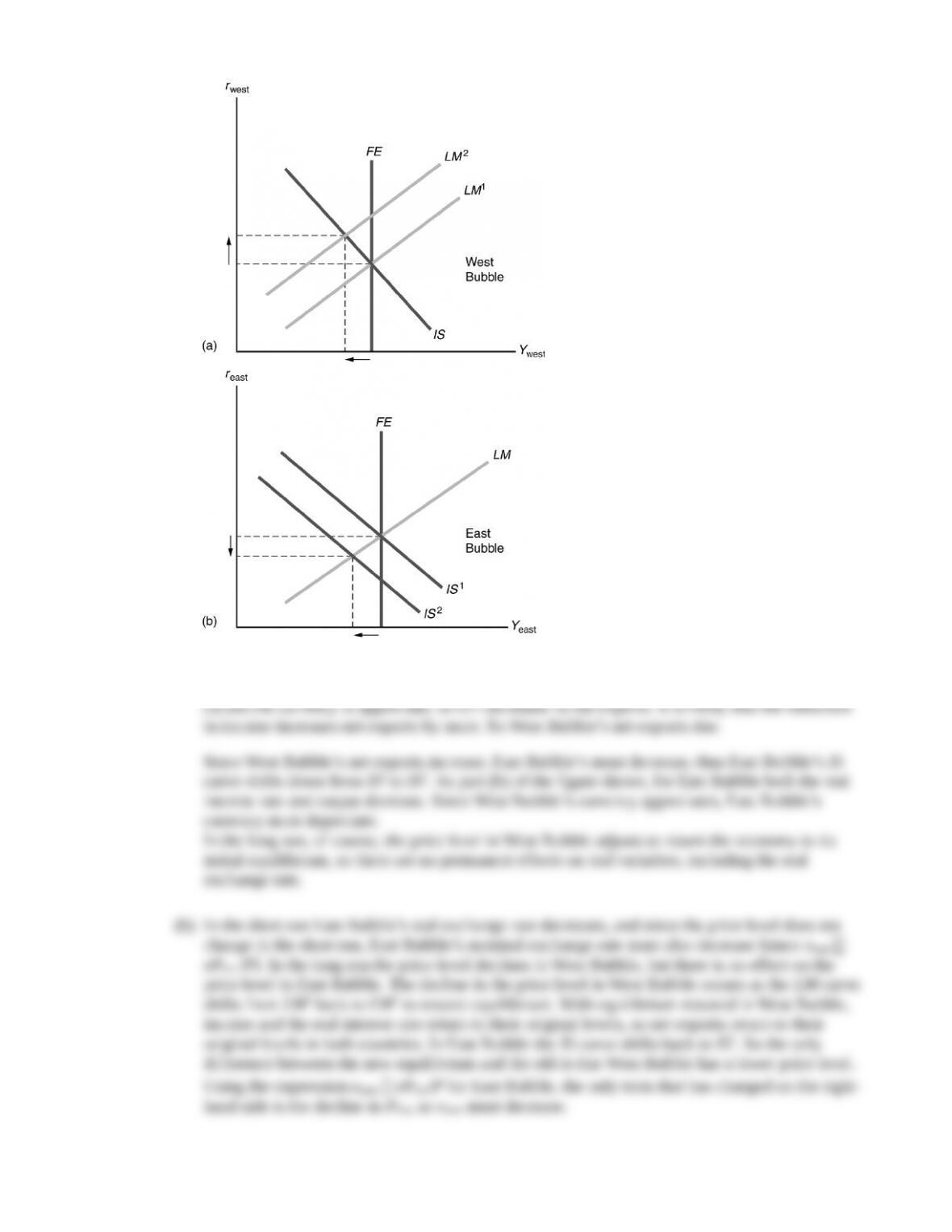
Figure 13.15
The decrease in West Bubble’s output increases its net exports. The higher real interest rate
4. (a) If people don’t want to spend more at a given real interest rate, they must increase desired
saving, so the S I curve shifts to the right. Since people aren’t spending more on imports, the
NX curve doesn’t shift. The new equilibrium is one with a lower real interest rate and higher net
exports.
(b) If people spend the full amount of the additional income, there will be no change in saving, so
IEB2, which passes through points F and H.
1. The nominal exchange rate is the rate at which two currencies can be exchanged for each other in the
market. The real exchange rate is the price of domestic goods relative to foreign goods. Changes in
2. The two major types of exchange-rate systems are fixed exchange rates and flexible exchange rates.
In a fixed-exchange-rate system, exchange rates are set at officially determined levels. In a flexible-
3. Purchasing power parity, PPP, is the idea that similar foreign and domestic goods, or baskets of
goods, should have the same price when priced in terms of the same currency. Purchasing power
4. The J curve shows the response of net exports to a real depreciation. At first the real depreciation
reduces net exports, as the decline in the real exchange rate means that a country pays more for its
5. An increase in domestic income leads people to buy more goods, including imported goods, so net
exports decline. An increase in foreign income leads foreigners to buy more goods, including goods
6. Foreigners demand dollars in the foreign exchange market to be able to buy U.S. goods and services
(U.S. exports) and U.S. real and financial assets (U.S. capital inflows). Americans supply dollars to
the foreign exchange market to be able to buy foreign goods and services (U.S. imports) and real and
financial assets in foreign countries (U.S. capital outflows). The demand for dollars increases if the
7. The IS–LM model for the open economy differs from the closed-economy IS–LM model in that
international influences may shift the IS curve. Factors that raise a country’s net exports, given
8. Expansionary fiscal policy increases output and the real interest rate in the short run (using a
Keynesian model), both of which lead to a reduction of net exports. Expansionary monetary policy
9. In the short run, expansionary monetary policy increases output (using a Keynesian model), which
decreases net exports, leading to an increased supply of the domestic currency in the foreign
exchange market, causing it to depreciate. Expansionary monetary policy also reduces the real
interest rate, causing reduced demand for domestic assets, again causing the currency to depreciate.
10. The fundamental value of a currency is the value of the exchange rate that would be determined by
free-market forces of demand and supply without government intervention. When the official
11.A country is limited in changing its money supply under a fixed-exchange-rate system, because
only one level of the money supply is consistent with the official exchange rate being equal to its
12. Flexible exchange rates have the advantage of allowing a country to use expansionary monetary
policy to combat recessions, but currency values fluctuate substantially, introducing uncertainty
into international transactions. Fixed exchange rates avoid this problem, but a country may have to
give up the independent use of monetary policy. This latter factor is a disadvantage when it comes
1. The price level in the West is PW 5 guilders per ordinary soap bar. The price level in the East is
PE 100 florins per deluxe soap bar. The real exchange rate is 2 ordinary soap bars per deluxe
soap bar.
(a) Use Eq. (13.6) to get enom ePFOR /P 2 ordinary soap bars per deluxe soap bar 5 guilders per
2. (a) Japan imports 64 barrels of oil, worth 16 cameras at 4 barrels of oil per camera. It exports
40 cameras, so the real value of its net exports is 24 cameras.
(b) Japan now imports 60 barrels of oil, worth 20 cameras at 3 barrels of oil per camera. It exports
42 cameras, so the real value of its net exports declines to 22 cameras.
(c) In the long run, Japan imports 54 barrels of oil, worth 18 cameras at 3 barrels of oil per camera.
3. Begin by writing the equation for the IS curve, which is Sd Id NX.
Sd Y Cd G Y (300 0.5Y 200r) G.
800r 640 0.6Y G.
(a) With G 100 and
Y
900, the IS curve gives 800r 640 540 100 200, so r 0.25.
Then e 20 600r 170, NX 150 90 85 25, C 300 450 50 700, and
4. (a) Begin by writing the equation for the IS curve, which is Sd Id NX.
NX 150 0.08Y 500r.
0.52Y (188 G) 200r (300 300r) 150 0.08Y 500r.
Rearranging terms and simplifying gives the IS curve:
1000r (638 G) 0.6Y.
The LM curve comes from the expression M/P L, which is 924/P 0.5Y 200r. In the long
run we’ll use this equation to find the price level, so we’ll write this as P 924/(0.5Y 200r).
In the short run we’ll combine the LM curve with the IS curve to find equilibrium, so we’ll write
0.6(1000 220) 38 630, and I 300 57 243.
(b) In the short run with G 214 and P 2, the IS curve now gives 1000r (638 214) 0.6Y,
0.24. Then NX 150 81.6 120 51.6, C 200 0.6(1020 224) 48 629.6, and I
300
72 228.
In the long run, using Y 1000 in the IS curve gives 1000r (638 214) (0.6 1000) 252,
10.4, while G is 62 lower, or 152. In the long run, NX is 62 higher than before (NX 6), while
G is 62 lower at 152.
5. (a) AD intersects AS at 1000 400 50M/P, which means M/P 12. With M 48 francs, P 4
francs/bottle. Use the formula enom ePFor /P 5 wedges/bottle 20 crowns/wedge/4 francs/
bottle 25 crowns/franc.
(b) At 50 crowns/franc, the franc is overvalued as the official rate exceeds the fundamental value.
6. (a) c0 200, cY 0.6, t0 20, t 0.2, cr 200
i0 300, ir 300
x0 150, xY 0.08, xYF 0, xr 500, xrF 0
r
IS IS
Ya b
¢ ¢
–
IS
a¢=
(c0 i0 G cYt0 x0 xYFYFor xrFrFor)/(cr ir xr)
(200 300 152 (0.6 20) 150 0 0)/(200 300 500)
790/1000 0.79
IS
b¢=
[1 (1 t)cY xY]/(cr ir xr)
[1 (1 0.2)0.6 0.08]/1000 0.0006
(b) r LM
(1/ )
r
l
M/P LMY
0
( / )
r
l l
/
l l
dominates, so net exports rise.
Suppose the economy is initially in a recession at the intersection of the IS1 and LM curves in
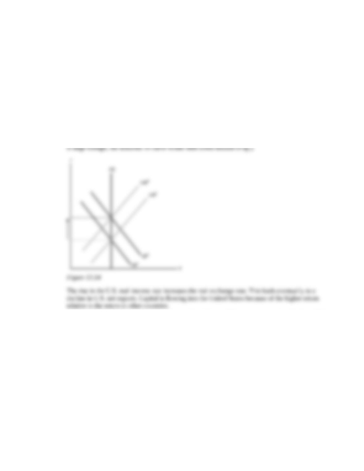
2. The fall in the MPKf abroad and the rise in the MPKf in the United States increases U.S. investment
for any given real interest rate, shifting the IS curve up and to the right. This is shown in Figure
13.14 as a shift from IS1 to IS2. To restore equilibrium, prices must rise so that the LM curve shifts up
from LM1 to LM2. At the new equilibrium the real interest rate is higher. So the result is an increase
in the price level, an increase in the real interest rate, and no change in output. (Note: The reduction
in MPKf abroad reduces investment abroad, leading to a decline in domestic net exports. If this effect
3. (a) West Bubble’s contractionary monetary policy shifts its LM curve up and to the left, from LM1
to LM2 in part (a) of Figure 13.15. The intersection of the IS and LM curves is one in which
output is below full-employment output and the real interest rate is higher than before.
Figure 13.15
The decrease in West Bubble’s output increases its net exports. The higher real interest rate
4. (a) If people don’t want to spend more at a given real interest rate, they must increase desired
saving, so the S I curve shifts to the right. Since people aren’t spending more on imports, the
NX curve doesn’t shift. The new equilibrium is one with a lower real interest rate and higher net
exports.
(b) If people spend the full amount of the additional income, there will be no change in saving, so
IEB2, which passes through points F and H.