3. Should the Fed Aim for Zero Inflation?
Discuss with your students the ultimate goal of the Federal Reserve (or any other country’s central bank). Should
the goal be to drive inflation to zero? Why is zero the best point to be? Is it good enough for inflation to be close
to zero, but positive, if it’s low and steady?
Here are some things to consider.
1. The Phillips curve is an empirical negative relationship between inflation and unemployment. The Phillips
curve relationship held for U.S. data in the 1960s, but broke down in the 1970s and 1980s.
2. In the traditional Phillips curve, inflation itself is related to the unemployment rate. In the expectations-
augmented Phillips curve, it is unanticipated inflation (the difference between actual
3. In the early 1960s the rate of inflation was fairly low (about 1% to 2%), and it didn’t vary much from year to
year. But supply shocks hit the economy in both the mid- and the late-1970s, causing a rise in expected
1980s. The instability of the Phillips curve is largely because of higher expected inflation associated with
supply shocks in the 1970s.
4. According to the classical point of view, the economy adjusts quickly to changes in inflation, so there is only
a very short period in which unemployment changes because of a change in inflation. Further, any
systematic attempt to reduce unemployment by increasing inflation would be fully anticipated, and would
have no effect on unemployment.
5. Policymakers want to keep inflation low because inflation imposes costs on the economy. Costs of
anticipated inflation include shoe leather costs and menu costs. Costs of unanticipated inflation include
6. The natural rate of unemployment is the rate of unemployment that exists when output is at its full-
employment level. This occurs when the only unemployment is frictional and structural, not cyclical. The
natural rate is crucial in understanding the Phillips curve
The natural rate of unemployment has moved higher over time in the United States and Europe due to a
number of factors. First, demographic changes occurred that raised the natural rate. Groups in the labor force
7. Two costs of anticipated inflation are shoe-leather costs and menu costs. Two costs of unanticipated inflation
are transfers of wealth and confusion of price signals.
8. The greatest potential cost of disinflation is that it may cause a recession. This occurs because inflation may
fall below expected inflation, causing the unemployment rate to rise along
9. One approach to disinflation is a cold turkey strategy. It has the advantage of reducing inflation quickly, but
it may have high costs from increasing unemployment, according to Keynesians.
10. The Federal Reserve works hard to establish its credibility so that the costs of reducing inflation
will be low. If the Federal Reserve has a great deal of credibility, then people will believe that the inflation
1. Since the natural rate of unemployment is 0.06, e 2(u 0.06), so u 0.06 0.5(e ),
or u 0.06 0.5(e ).
2 0.02 0.04, or 4%.
Year 2: u 0.06 0.5(0.04 0.04) 0.06. The unemployment rate equals the natural rate, since
inflation equals expected inflation. Since unemployment is at its natural rate, output is at its
full-employment level.
1 0.08 0.10 0.07 0.01 0.02
2 0.04 0.08 0.08 0.02 0.04
3 0.04 0.06 0.07 0.01 0.02
4 0.04 0.04 0.06 0.0 0.0
The total output shortfall is 0.02 0.04 0.02 0.0 0.08 8-percentage points of output lost.
2. (a) Equating aggregate demand to short-run aggregate supply gives: 300 10(M/P) 500 P Pe, or 300
(10 1000/P) 500 P 50, or 10,000/P 150 P. Multiplying both sides of the equation by P
and rearranging gives P2 150P 10,000 0, which can be factored as (P 50)
(P 200) 0. This has the nonnegative solution P 50. Since Pe is also 50, the expected price level
equals the actual price level, so output is at its full-employment level of 500 and the unemployment rate
500)/500 0.02. With a natural unemployment rate of 0.06, Okun’s Law gives 0.02 2(u 0.06).
This can be solved to get u 0.05.
In the long run, Pe adjusts to equal P, output adjusts to its full-employment level of 500, and
unemployment adjusts to the natural rate of 0.06. To find P, use the aggregate demand curve
3. (a) 0.10 2(u 0.06) 0.22 2u. This is shown as the Phillips curve labeled PCa in Figure 12.6. If the
Fed keeps inflation at 0.10, then u 0.06, the natural rate of unemployment.
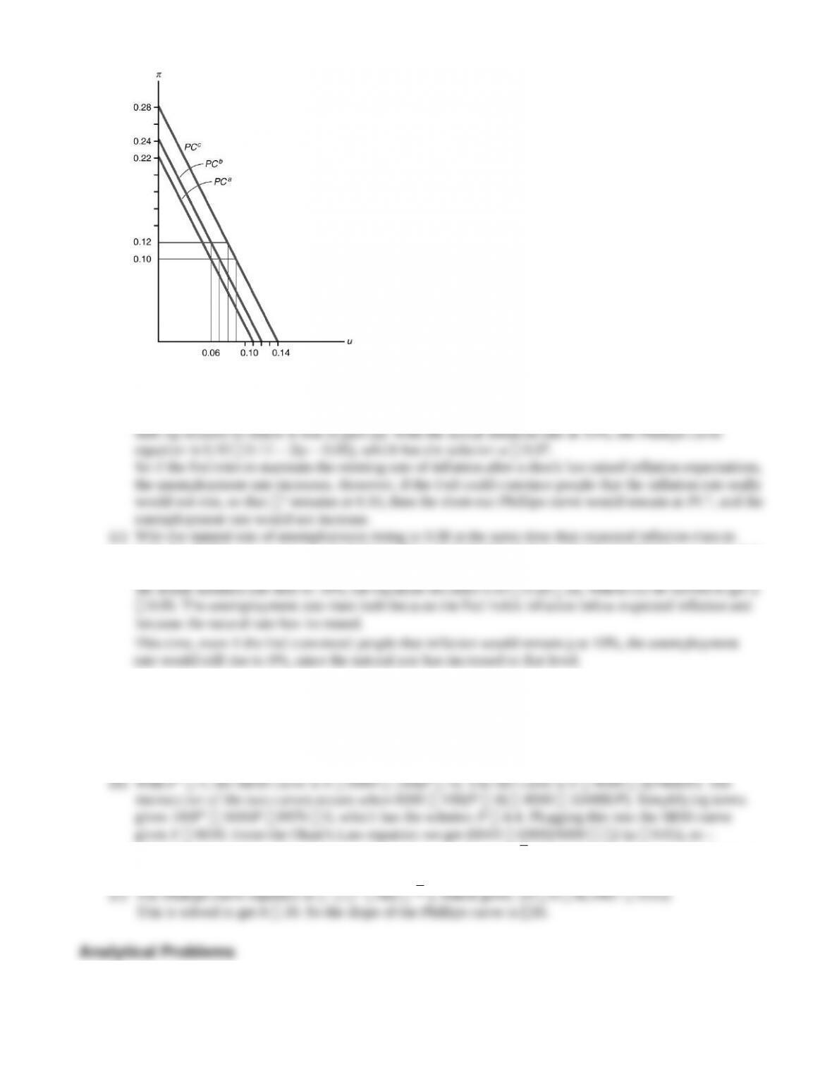
Figure 12.6
(b) With expected inflation rising to 12%, the Phillips curve is 0.12 – 2(u – 0.06) 0.24 – 2u. This is
the Phillips curve labeled PCb in the figure. The higher rate of expected inflation has caused the curve to
0.12, the Phillips curve equation is 0.12 2(u 0.08) 0.28 2u. This is the Phillips curve labeled
PCc in the figure. The new short-run Phillips curve is even higher than those for parts (a) and (b). With
4. (a) Beginning in long-run equilibrium, with M 4000, output must be at its full-employment level
of 6000 and the unemployment rate must be equal to the natural rate of .05. Using the values for Y and
M in the AD curve, 6000 4000 2(4000/P), which gives P 4. This is also the expected price level.
Because M has been constant for a long time and is expected to remain constant,
e 0.
0.00333 u 0.05, so u .0467. Cyclical unemployment is u
u
0.0033. Unanticipated inflation is
(P Pe)/Pe 0.10 10%.
u
1. (a) The reduction in structural unemployment would reduce the natural rate of unemployment and thus
would shift both the expectations-augmented Phillips curve and the long-run Phillips curve to the left.

2. The slope of the short-run aggregate supply curve will be much steeper in economy B, because producers
increase their output only a small amount in response to an increase in price. But economy A’s short-run
3. (a) In Figure 12.7, the SRAS curve shifts up 10% each year, as does the AD curve. Unanticipated inflation is
zero, as both actual and expected inflation are 10%. The economy is at full employment, since firms set
their prices to exactly match the increase in the general price level.
Figure 12.7
(b) The surprise increase in the money supply at mid-year leads to a rise in output, as shown in Figure 12.8
4. In the cashless society, there would be no shoe-leather costs, as there would be no cash balances
on which to economize. But menu costs would remain for anticipated inflation. The costs of unanticipated
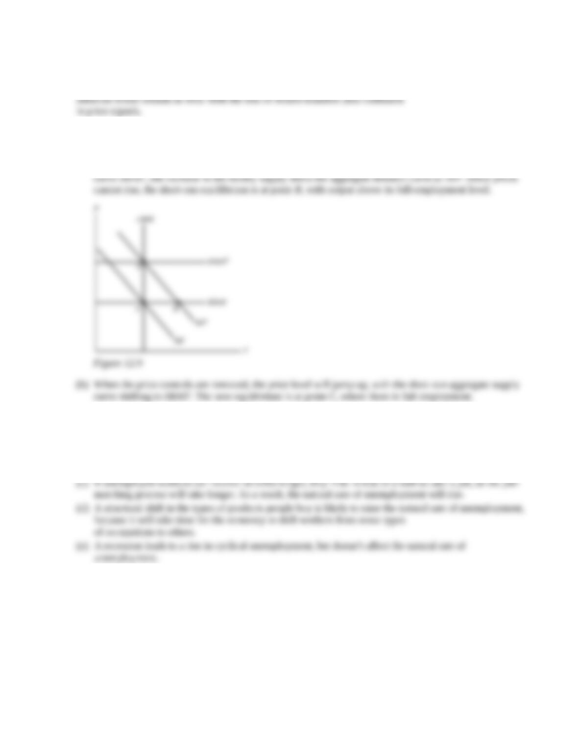
5. (a) Figure 12.9 shows the effects of increasing the money supply while holding the price level constant.
Beginning at point A, the intersection of aggregate demand curve AD1 and short-run aggregate supply
6. (a) A new law that prohibits people from seeking employment before age eighteen is likely to reduce the
natural rate of unemployment because teenagers have a higher-than-average unemployment rate. With no
teenagers allowed in the labor force, the average unemployment rate would be lower.
(b) A service that makes looking for a job easier is able to match people and jobs more rapidly, which
should reduce the natural rate of unemployment.
Here are some things to consider.
1. The Phillips curve is an empirical negative relationship between inflation and unemployment. The Phillips
curve relationship held for U.S. data in the 1960s, but broke down in the 1970s and 1980s.
2. In the traditional Phillips curve, inflation itself is related to the unemployment rate. In the expectations-
augmented Phillips curve, it is unanticipated inflation (the difference between actual
3. In the early 1960s the rate of inflation was fairly low (about 1% to 2%), and it didn’t vary much from year to
year. But supply shocks hit the economy in both the mid- and the late-1970s, causing a rise in expected
1980s. The instability of the Phillips curve is largely because of higher expected inflation associated with
supply shocks in the 1970s.
4. According to the classical point of view, the economy adjusts quickly to changes in inflation, so there is only
a very short period in which unemployment changes because of a change in inflation. Further, any
systematic attempt to reduce unemployment by increasing inflation would be fully anticipated, and would
have no effect on unemployment.
5. Policymakers want to keep inflation low because inflation imposes costs on the economy. Costs of
anticipated inflation include shoe leather costs and menu costs. Costs of unanticipated inflation include
6. The natural rate of unemployment is the rate of unemployment that exists when output is at its full-
employment level. This occurs when the only unemployment is frictional and structural, not cyclical. The
natural rate is crucial in understanding the Phillips curve
The natural rate of unemployment has moved higher over time in the United States and Europe due to a
number of factors. First, demographic changes occurred that raised the natural rate. Groups in the labor force
7. Two costs of anticipated inflation are shoe-leather costs and menu costs. Two costs of unanticipated inflation
are transfers of wealth and confusion of price signals.
8. The greatest potential cost of disinflation is that it may cause a recession. This occurs because inflation may
fall below expected inflation, causing the unemployment rate to rise along
9. One approach to disinflation is a cold turkey strategy. It has the advantage of reducing inflation quickly, but
it may have high costs from increasing unemployment, according to Keynesians.
10. The Federal Reserve works hard to establish its credibility so that the costs of reducing inflation
will be low. If the Federal Reserve has a great deal of credibility, then people will believe that the inflation
1. Since the natural rate of unemployment is 0.06, e 2(u 0.06), so u 0.06 0.5(e ),
or u 0.06 0.5(e ).
2 0.02 0.04, or 4%.
Year 2: u 0.06 0.5(0.04 0.04) 0.06. The unemployment rate equals the natural rate, since
inflation equals expected inflation. Since unemployment is at its natural rate, output is at its
full-employment level.
1 0.08 0.10 0.07 0.01 0.02
2 0.04 0.08 0.08 0.02 0.04
3 0.04 0.06 0.07 0.01 0.02
4 0.04 0.04 0.06 0.0 0.0
The total output shortfall is 0.02 0.04 0.02 0.0 0.08 8-percentage points of output lost.
2. (a) Equating aggregate demand to short-run aggregate supply gives: 300 10(M/P) 500 P Pe, or 300
(10 1000/P) 500 P 50, or 10,000/P 150 P. Multiplying both sides of the equation by P
and rearranging gives P2 150P 10,000 0, which can be factored as (P 50)
(P 200) 0. This has the nonnegative solution P 50. Since Pe is also 50, the expected price level
equals the actual price level, so output is at its full-employment level of 500 and the unemployment rate
500)/500 0.02. With a natural unemployment rate of 0.06, Okun’s Law gives 0.02 2(u 0.06).
This can be solved to get u 0.05.
In the long run, Pe adjusts to equal P, output adjusts to its full-employment level of 500, and
unemployment adjusts to the natural rate of 0.06. To find P, use the aggregate demand curve
3. (a) 0.10 2(u 0.06) 0.22 2u. This is shown as the Phillips curve labeled PCa in Figure 12.6. If the
Fed keeps inflation at 0.10, then u 0.06, the natural rate of unemployment.
Figure 12.6
(b) With expected inflation rising to 12%, the Phillips curve is 0.12 – 2(u – 0.06) 0.24 – 2u. This is
the Phillips curve labeled PCb in the figure. The higher rate of expected inflation has caused the curve to
0.12, the Phillips curve equation is 0.12 2(u 0.08) 0.28 2u. This is the Phillips curve labeled
PCc in the figure. The new short-run Phillips curve is even higher than those for parts (a) and (b). With
4. (a) Beginning in long-run equilibrium, with M 4000, output must be at its full-employment level
of 6000 and the unemployment rate must be equal to the natural rate of .05. Using the values for Y and
M in the AD curve, 6000 4000 2(4000/P), which gives P 4. This is also the expected price level.
Because M has been constant for a long time and is expected to remain constant,
e 0.
0.00333 u 0.05, so u .0467. Cyclical unemployment is u
u
0.0033. Unanticipated inflation is
(P Pe)/Pe 0.10 10%.
u
1. (a) The reduction in structural unemployment would reduce the natural rate of unemployment and thus
would shift both the expectations-augmented Phillips curve and the long-run Phillips curve to the left.
2. The slope of the short-run aggregate supply curve will be much steeper in economy B, because producers
increase their output only a small amount in response to an increase in price. But economy A’s short-run
3. (a) In Figure 12.7, the SRAS curve shifts up 10% each year, as does the AD curve. Unanticipated inflation is
zero, as both actual and expected inflation are 10%. The economy is at full employment, since firms set
their prices to exactly match the increase in the general price level.
Figure 12.7
(b) The surprise increase in the money supply at mid-year leads to a rise in output, as shown in Figure 12.8
4. In the cashless society, there would be no shoe-leather costs, as there would be no cash balances
on which to economize. But menu costs would remain for anticipated inflation. The costs of unanticipated
5. (a) Figure 12.9 shows the effects of increasing the money supply while holding the price level constant.
Beginning at point A, the intersection of aggregate demand curve AD1 and short-run aggregate supply
6. (a) A new law that prohibits people from seeking employment before age eighteen is likely to reduce the
natural rate of unemployment because teenagers have a higher-than-average unemployment rate. With no
teenagers allowed in the labor force, the average unemployment rate would be lower.
(b) A service that makes looking for a job easier is able to match people and jobs more rapidly, which
should reduce the natural rate of unemployment.