Figure 11.15 Figure 11.16
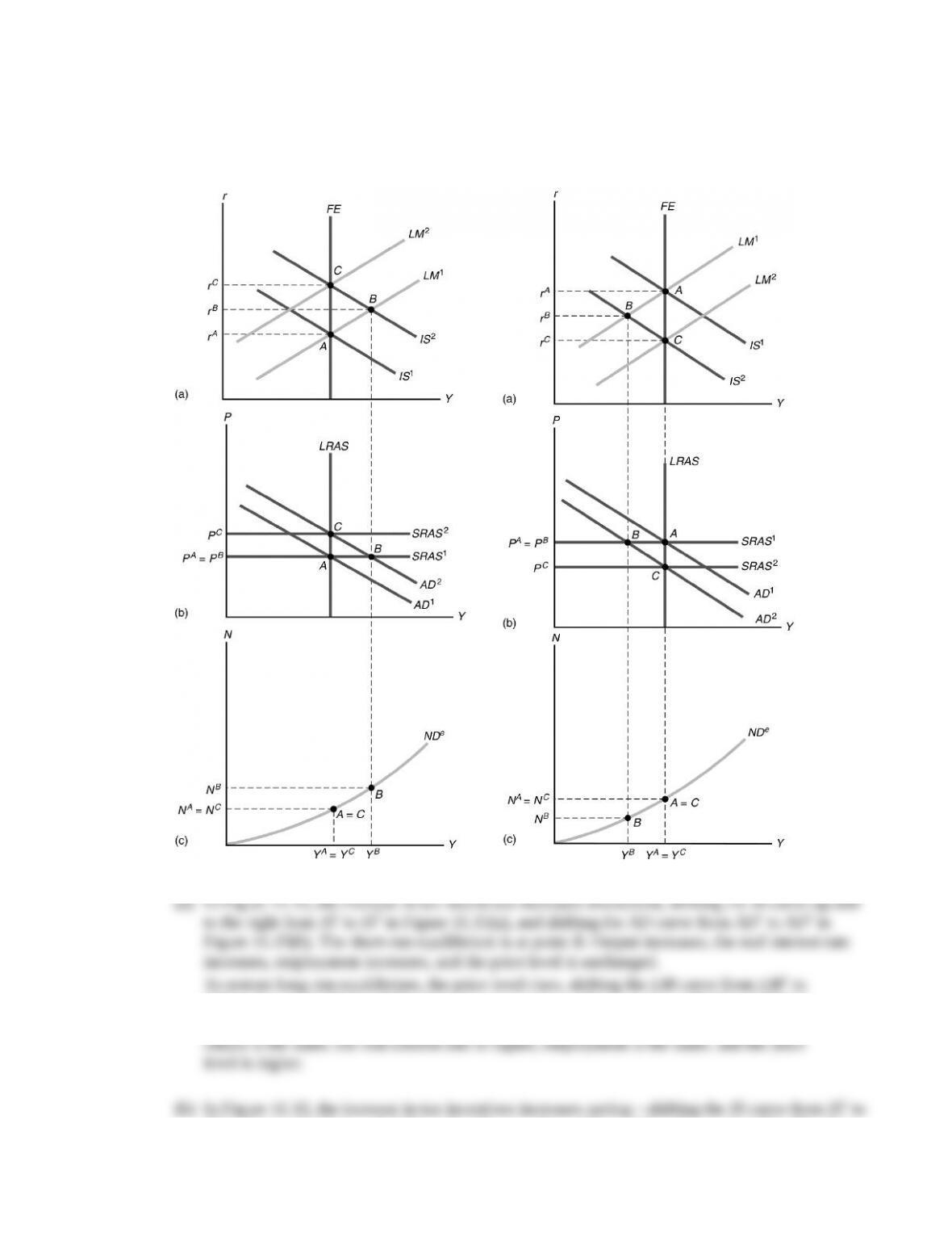
LM2 in Figure 11.15(a) and the short-run aggregate supply curve from SRAS1 to SRAS2 in
Figure 11.15(b). The long-run equilibrium is at point C. Compared to the starting point,
IS2 in Figure 11.16(a), and shifting the AD curve from AD1 to AD2 in Figure 11.16(b). The short-
run equilibrium is at point B. Output decreases, the real interest rate decreases, employment
decreases, and the price level is unchanged.
To restore long-run equilibrium, the price level declines, shifting the LM curve from LM1
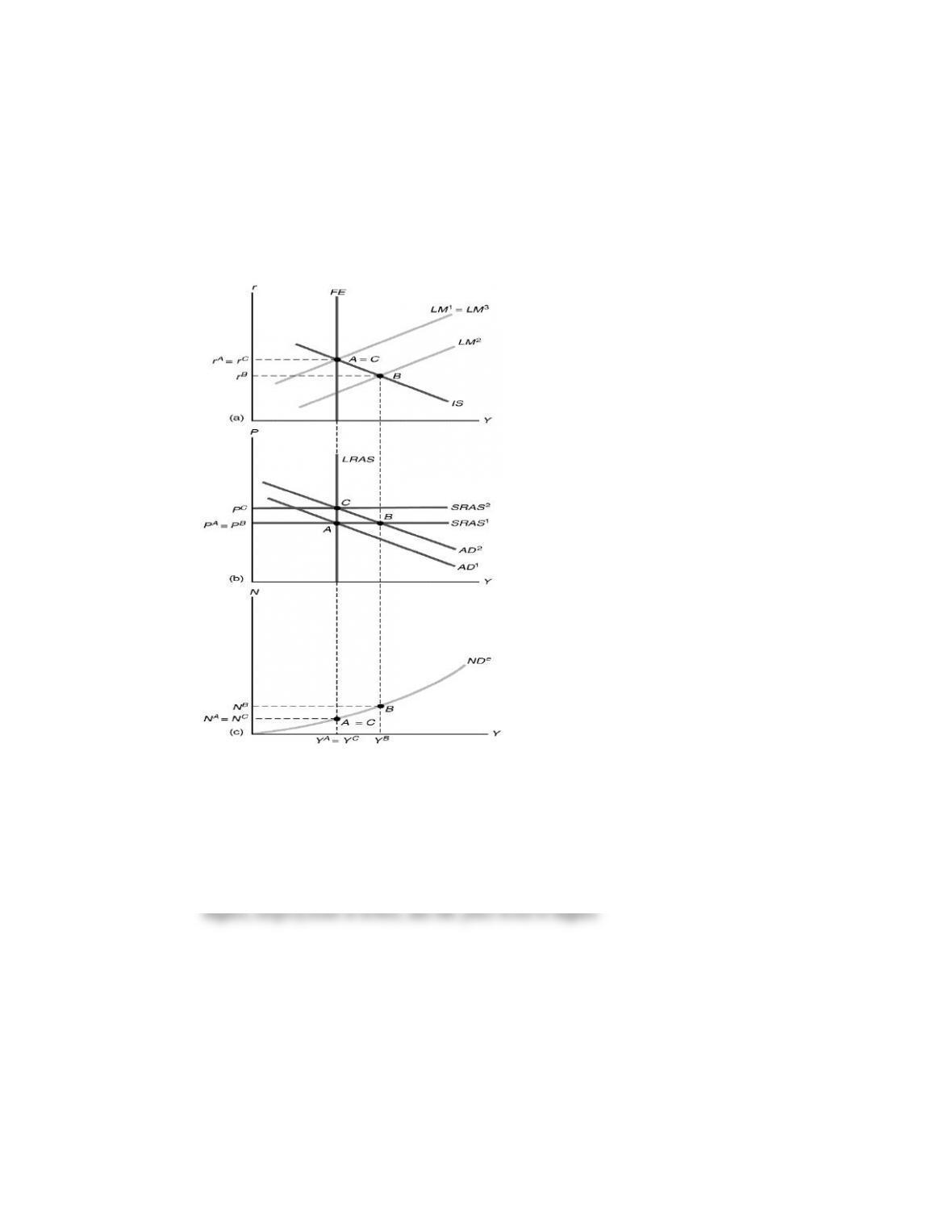
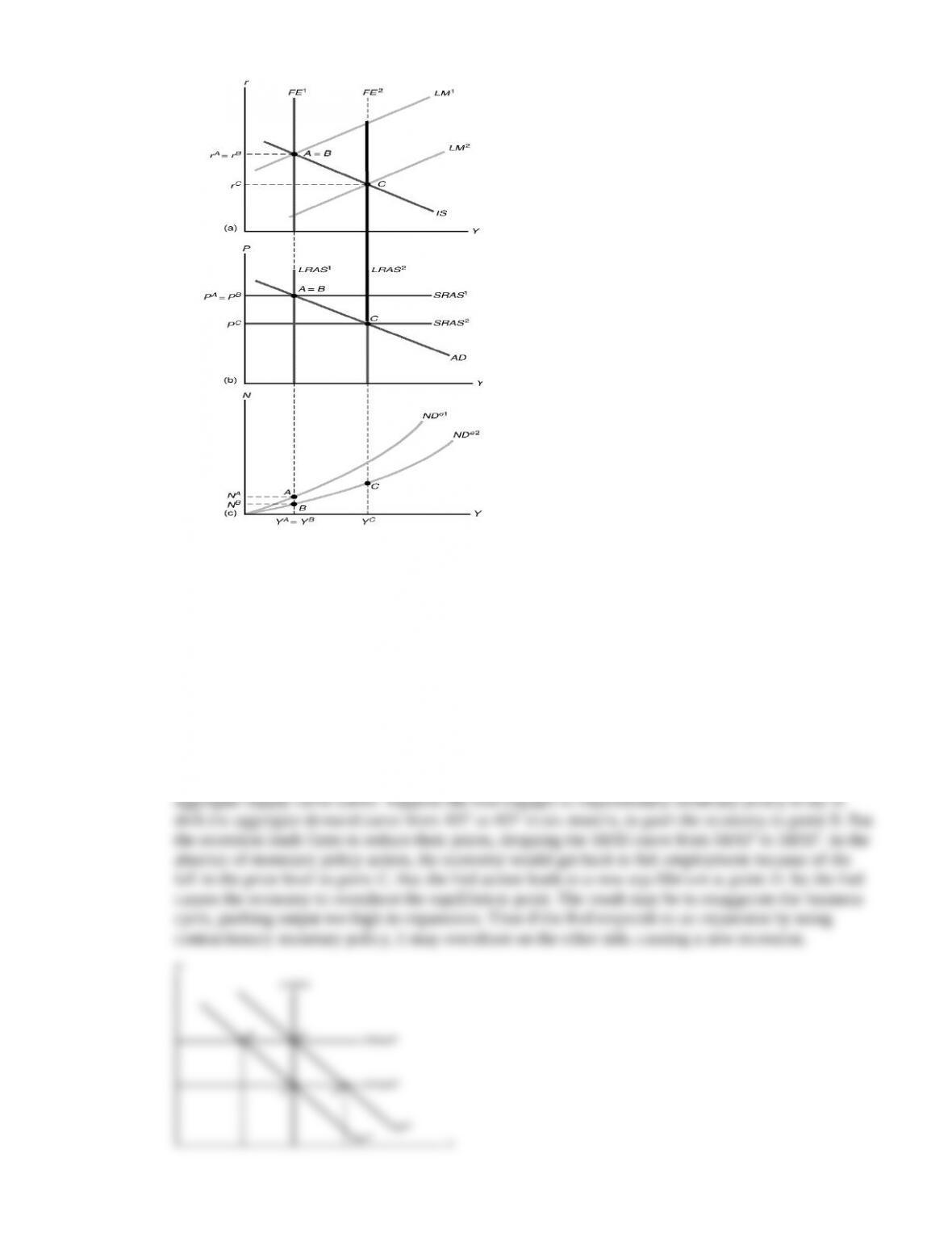
2. In Figures 11.17–11.20, point A is the starting point, point B shows the short-run equilibrium after
the change, and point C shows the long-run equilibrium after the change.
(a) In Figure 11.17, when banks pay a higher interest rate on checking accounts, the demand for
money rises, shifting the LM curve up and to the left from LM1 to LM2 in Figure 11.17(a). As a
result, the AD curve shifts down and to the left from AD1 to AD2 in Figure 11.17(b). The new
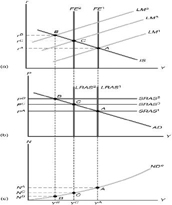
FE2, and shifts the LRAS line from LRAS1 to LRAS2. The rise in agricultural prices increases the
price level, so the short-run aggregate supply curve shifts up from SRAS1 to SRAS2. Also, the rise
in the price level shifts the LM curve up and to the left from LM1 to LM2. The short-run equilibrium
is at point B, assuming that the LM curve shifts so much that it intersects the IS curve to the left
of the FE line. At point B, compared to the starting point, output is lower, the real interest rate is
3. A lag in the impact of policy of six months, which is about the time it takes firms to adjust prices,
could cause policy to be destabilizing. That is, monetary policy may be pushing the economy away
from equilibrium.
To see this, suppose the economy is in a recession at point A in Figure 11.21. The short-run aggregate
supply curve SRAS1 intersects the aggregate demand curve AD1 at point A, to the left of the long-run
4. An increase in government purchases shifts the IS curve up and to the right and the AD curve up and
to the right to return the economy to full employment, instead of waiting for the price level to fall to
get there. The advantage of doing so, according to Keynesians, is that full employment is restored
quickly, whereas if the price level must adjust, it may take a long time for full employment to be
restored. In the short run, the fiscal expansion does not affect the real wage, since it is an efficiency
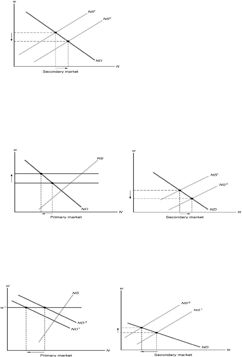
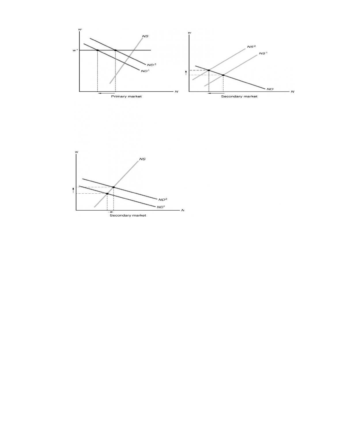
5. (a) In response to expansionary monetary policy, aggregate demand increases, increasing output and
labor demand. This causes the labor demand curve to shift from ND1 to ND2 in the primary labor
market, shown in Figure 11.22. The result is an increase in employment and output with no
change in the real wage in the primary labor market. Since more workers are now in the primary
labor market, the labor supply in the secondary labor market decreases from NS1 to NS2. This causes
run equilibrium is at point B. Output decreases, the real interest rate decreases, employment
decreases, and the price level is unchanged.
To restore long-run equilibrium, the price level declines, shifting the LM curve from LM1
2. In Figures 11.17–11.20, point A is the starting point, point B shows the short-run equilibrium after
the change, and point C shows the long-run equilibrium after the change.
(a) In Figure 11.17, when banks pay a higher interest rate on checking accounts, the demand for
money rises, shifting the LM curve up and to the left from LM1 to LM2 in Figure 11.17(a). As a
result, the AD curve shifts down and to the left from AD1 to AD2 in Figure 11.17(b). The new
FE2, and shifts the LRAS line from LRAS1 to LRAS2. The rise in agricultural prices increases the
price level, so the short-run aggregate supply curve shifts up from SRAS1 to SRAS2. Also, the rise
in the price level shifts the LM curve up and to the left from LM1 to LM2. The short-run equilibrium
is at point B, assuming that the LM curve shifts so much that it intersects the IS curve to the left
of the FE line. At point B, compared to the starting point, output is lower, the real interest rate is
3. A lag in the impact of policy of six months, which is about the time it takes firms to adjust prices,
could cause policy to be destabilizing. That is, monetary policy may be pushing the economy away
from equilibrium.
To see this, suppose the economy is in a recession at point A in Figure 11.21. The short-run aggregate
supply curve SRAS1 intersects the aggregate demand curve AD1 at point A, to the left of the long-run
4. An increase in government purchases shifts the IS curve up and to the right and the AD curve up and
to the right to return the economy to full employment, instead of waiting for the price level to fall to
get there. The advantage of doing so, according to Keynesians, is that full employment is restored
quickly, whereas if the price level must adjust, it may take a long time for full employment to be
restored. In the short run, the fiscal expansion does not affect the real wage, since it is an efficiency
5. (a) In response to expansionary monetary policy, aggregate demand increases, increasing output and
labor demand. This causes the labor demand curve to shift from ND1 to ND2 in the primary labor
market, shown in Figure 11.22. The result is an increase in employment and output with no
change in the real wage in the primary labor market. Since more workers are now in the primary
labor market, the labor supply in the secondary labor market decreases from NS1 to NS2. This causes