978-0132992282 Chapter 11 Solution Manual Part 1

Type Homework Help

Pages 13

Words 3174

Textbook Macroeconomics 8th Edition

Authors Andrew B. Abel, Ben Bernanke, Dean Croushore

Unlock document.

This document is partially blurred.

Unlock all pages and 1 million more documents.

Get Access

Additional Issues for Classroom Discussion

1. Do Lags Eliminate the Effectiveness of Fiscal Policy?

Keynesian economists in the past have encouraged the use of fiscal policy to combat recession. They

believe that wages and prices do not adjust rapidly enough to bring the economy to full employment in a

reasonable period of time without the help of changes in government expenditures. However, fiscal policy

takes a long time to be implemented. Can we expect it to be effective in combating recessions?

2. Do Prices Adjust Slowly?

One of the main differences between Keynesians and classical economists is their disagreement over how

quickly prices adjust to changes in the economy. Which point of view seems more in line with what

happens in the economy?

In some markets, prices do adjust rapidly. This is particularly true in commodity markets such as those for

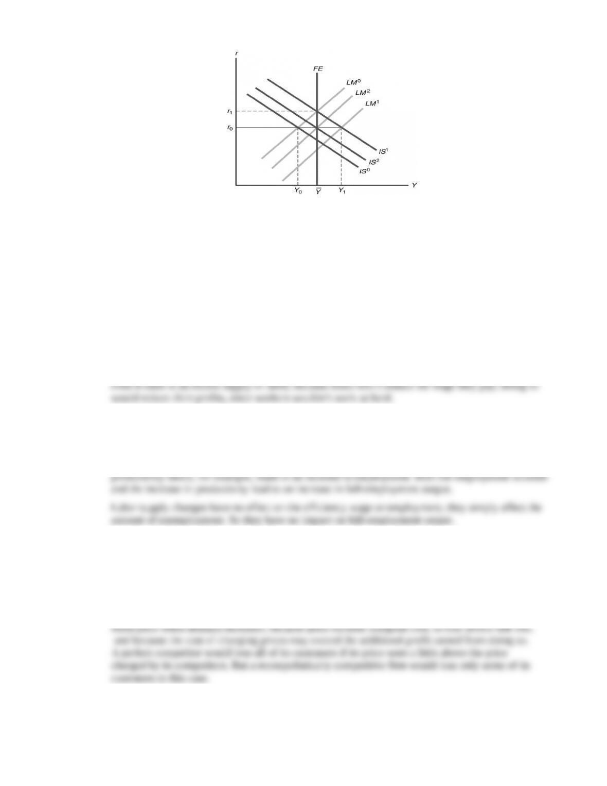
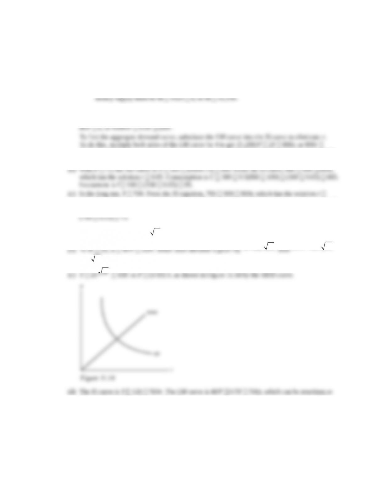
3. The Interest Rate Forecast for 1993

In late 1992, private forecasters suggested that the Fed would need to raise interest rates in 1993 as the

economy expanded. This can be seen in Figure 11.10, in which the economy is initially in equilibrium with

the IS curve at IS0 and the LM curve at LM0. The forecast for 1993 was that the IS curve would shift up

and to the right to I S1. If the Fed maintained the real interest rate at r0, it would need to expand the money

supply to shift the LM curve to LM1, which would increase output beyond the full-employment level. To

prevent this, the Fed would have to allow interest rates to rise to r1.

1. The efficiency wage is the real wage that maximizes effort or efficiency per dollar of real wages. It

assumes that workers will exert more effort, the higher the real wage. The real wage will remain rigid

2. Full-employment output is the amount of output produced by firms with employment determined by

the labor demand curve at the point where the marginal product of labor equals the efficiency wage.

A productivity shock does not lead to a change in the efficiency wage, since it does not affect work

effort. But it does affect the marginal product of labor, so employment changes. A beneficial

3. Price stickiness is the tendency of prices to adjust only slowly to changes in the economy. Keynesians

believe it is important to allow for price stickiness to explain why monetary policy is not neutral.

4. Menu costs are the costs of changing prices. Menu costs may lead to price stickiness in

monopolistically competitive markets but not in perfectly competitive markets, because a

monopolistically competitive firm’s demand is not as sensitive to the price as is a perfectly

competitive firm’s demand. Monopolistically competitive firms may meet the demand at a

5. In the Keynesian model, money is not neutral in the short run, but it is neutral in the long run. In

the short run, an increase in the money supply increases output and the real interest rate, while the

price level and real (efficiency) wage are unchanged. In the long run, however, only the price level

is changed, with no change in output, the real interest rate, or the real wage. In the basic classical

6. In the Keynesian model in the short run, output and the real interest rate increase due to an increase

in government purchases. In the long run, the real interest rate is higher, but output returns to its full-

7. In response to a recession, policymakers can (1) make no change in macroeconomic policy,

(2) increase the money supply, or (3) increase government purchases.

If they make no change in macroeconomic policy, then during the recession output is below its

full-employment level. Over time, the price level will decline to restore equilibrium. In the long run,

the price level will be lower and employment will return to the full-employment level.

8. Employment is procyclical because a contractionary aggregate demand shock reduces both output

and employment. Money is procyclical because price stickiness means that an increase in the money

supply increases output as the aggregate demand curve moves along the flat, short-run, aggregate

supply curve. Inflation is procyclical, because in a recession the price level declines over time to

9. The Keynesian theory assumes that demand shocks cause most cyclical fluctuations. This means that

during expansions when employment rises, average labor productivity declines, so it is countercyclical.

10. In Keynesian analysis, a supply shock may reduce output in two ways: (1) a reduction in output,

because the supply shock reduces the marginal product of labor, shifting the FE line to the left; and

(2) a further reduction in output if the supply shock is something like an oil price shock that is large

enough to cause many firms to raise prices, shifting the LM curve up and to the left so much that it

1. The following table shows the real wage (w), the effort level (E), and the effort per unit of real wages

(E/w).

8 7 0.875

10 10 1.00

12 15 1.25

14 17 1.21

16 19 1.19

18 20 1.11

The firm will pay a wage of 12, since that wage provides the maximum effort per unit of the real

2. (a) The IS curve is found from the equation Y  Cd  Id  G  130  0.5(Y  100)  500r  100 

500r  100, or 0.5Y  280  1000r, or Y  560  2000r.

The LM curve comes from the equation M/P  L, which in this case is 1320/P  0.5Y  1000r,

100)  500r  130  0.5(500  100)  (500  0.03)  315. Investment is I  100  (500  0.03)

 85.

100, or 0.5Y  380  1000r, or Y  760  2000r. In the short run, the price level remains fixed at

6, so the LM curve remains at LM1. With the price level equal to 6, the LM curve has the equation

Y  (2640/P)  2000r  440  2000r. The IS and LM curves intersect where 760  2000r  440 

2000r, or 320  4000r, which has the solution r  0.08. At r  0.08, output is given from the

IS curve as Y  760  2000r  760  (2000  0.08)  600. Then consumption is C  130  0.5

200  (500  0.08)  160.

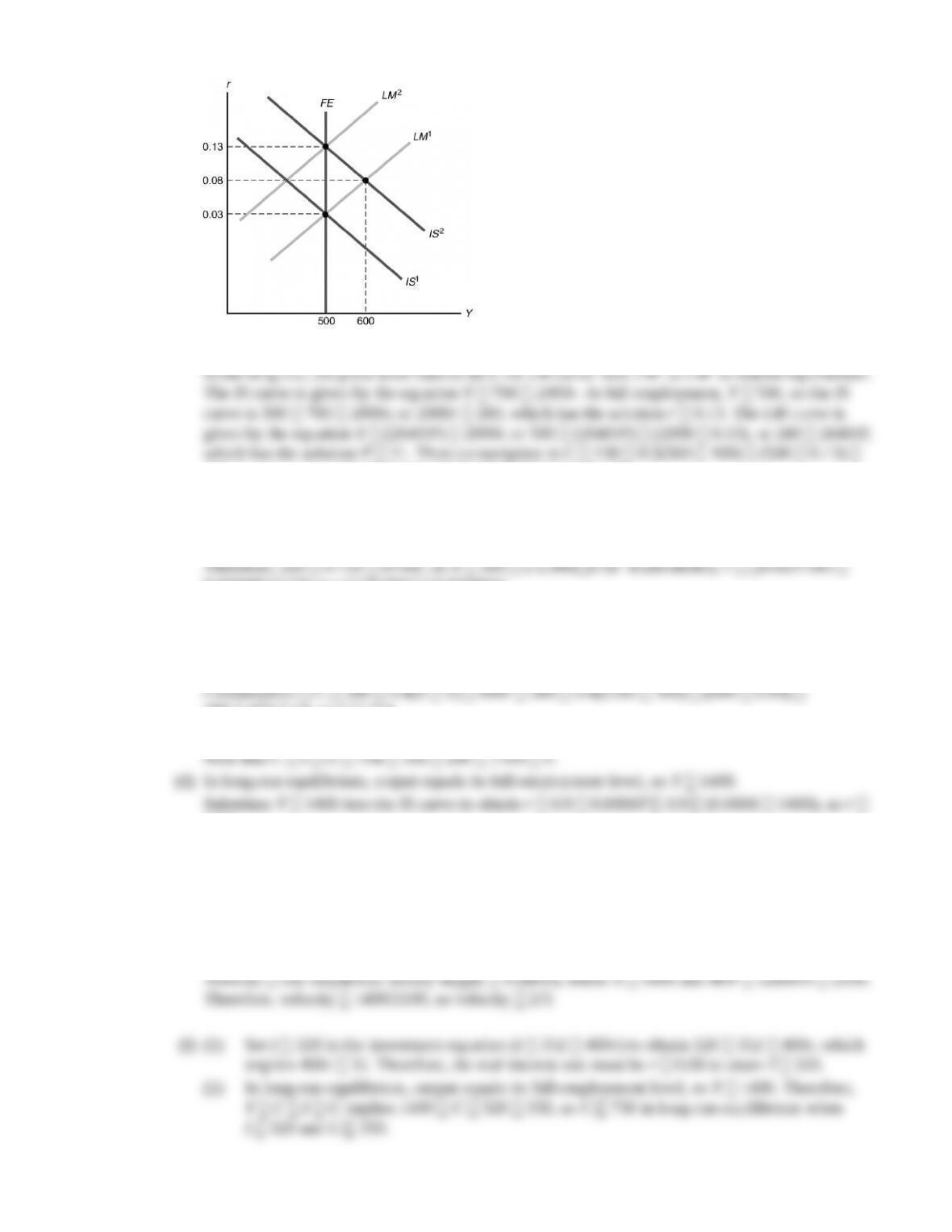
Figure 11.11

265. Investment is I  200  500r  200  (500  0.13)  135.

3. (a) Y  C  I  G  [388  0.4(Y  300)  600r]  [352  400r]  280  900  0.4Y  1000r,

so 0.6Y  900  1000r. Therefore, Y  1500  (1666  2/3)r. Equivalently, r  0.9  0.0006Y.

(b) 12600/7  M/P  L  1750  0.75Y  8750(r  0.02), so 1800  1750  0.75Y  8750r  175.

0.0000857143Y or r  9/350  (3/35000)Y.

1/3)r. Therefore, r  0.09. Substitute r  0.09 into the IS curve to obtain Y  1500  [(16662/3) 

0.09], so Y  1350. As a check, you can substitute r  0.09 into the equation for the LM curve, to

obtain Y  300  [(11,666  2/3)  0.09]  1350.

388  420  54, so C  754.

Investment  I  352  400r  352  (400  0.09), so I  316.

0.06.

Consumption  C  388  0.4(Y  T)  600r  388  0.4(1400  300)  (600  0.06), so C 

792.

Investment  I  352  400r  352  (400  0.06), so I  328.

Note that C  I  G  792  328  280  1400  Y.

(e) M/P  L, so P = M/L  12,600/[1750  0.75Y  8750(r  e)]  12,600/{1750  (0.75  1400) 

[8750(0.06  0.02)]} 12,600/2100, so P  6.

350.

(4) In long-run equilibrium, Y  1400 and r  0.08, so L  1750  0.75Y  8750(r  e) 

1750  (0.75  1400)  [8750  (0.08  0.02)]  1925. Since M/P = L  1925, we have M

 1925  P. To attain P  6 in long-run equilibrium with I  320 and G  350, the nominal

4. (a) The IS curve is given by Y  Cd  Id  G  300  0.5(Y  100)  300r  100  100r  100  450

 0.5Y  400r. This can be rewritten as 0.5Y  450  400r, or Y  900  800r. The LM curve is

2Y  (25,200/P). Then substitute this in the IS curve: Y  900  800r  900  [2Y  (25,200/P)].

This can be rewritten as 3Y  900  (25,200/P), or Y  300  (8400/P).

0.25. The LM curve then is 6300/P  (0.5  700)  (200  0.25)  300, which has the solution P

 21. Consumption is C  300  0.5(700  100)  (300  0.25)  525. Investment is I  100 

5. (a) Setting w  MPN,

10/ .w N=

This is the labor demand curve.

10/ ,w N=

20/ 10/ ,P N=

or 2

 P.

 10P, or P  (1/10) Y, as shown in Figure 11.14 by the SRAS curve.

Figure 11.14

(d) The IS curve is Y  120  500r. The LM curve is M/P  0.5Y  500r, which can be rewritten as

500r  0.5Y  (M/P). Plugging the LM curve into the IS curve to eliminate r gives Y  120 

500r  120  [0.5Y  (M/P)]. This can be rewritten as 1.5Y  120  (M/P). This is the AD curve.

With M  300, the AD curve is 1.5Y  120  (300/P), or Y  80  (200/P). The AD curve is

shown in Figure 11.14.

(e) To find the intersection of the SRAS curve (Y  10P) and the AD curve [Y  80  (200/P)], find

the price level such that 10P  80  (200/P). This can be rewritten as 10P2  80P  200  0, or

20/10  2.

(f) When the money supply falls to 135, the AD curve becomes 1.5Y  120  (135/P), or Y  80 

as 10P2  80P  90  0, or P2  8P  9  0. This can be factored as (P  9)(P  1)  0, which

has the nonnegative solution P  9. From the SRAS curve, Y  10P  10  9  90. From the IS

20.25.

The real wage is w  W/P  20/9  2 2/9.

6. (a) Y  Cd  Id  G  [325  0.5(1000  150)  500r]  [200  500r]  150, so 1000r  100,

so r  0.10.

M/P  L, so 6000/P  0.5Y  1000r  (0.5  1000)  (1000  0.10)  400, so P  15.

C  325  0.5(Y  T)  500r  325  0.5(1000  150)  (500  .10)  700.

1.1/.001  1100.

(e) Y/G  1/[(cr  ir)(IS  LM)]  1/[(500  500)(.0005  .0005)]  1.