
Additional Issues for Classroom Discussion
1. Do Wages Adjust to Clear the Labor Market?
One of the key assumptions of classical macroeconomic theory is that wages adjust rapidly to bring about
equilibrium in the labor market in a relatively short period of time. Is this a reasonable assumption?
Some economists look at the labor-market statistics, which show large swings in unemployment and
not much change in wages over the business cycle. They believe this indicates sluggish wage adjustment,
2. Are People ’s Inflation Forecasts Rational?
When the misperceptions theory was developed in the late 1970s, a number of economists began testing
people’s forecasts to see how rational they were. The theory implies that on average, people should not
make systematic errors in forecasting. Of special importance are people’s forecasts of inflation, since
these affect the aggregate supply curve.
provided their forecasts for surveys didn’t have a strong incentive to forecast rationally. They weren’t
investors with money at risk if their forecasts turned out to be wrong. And even if they did have money
on the line, they might not have provided their true forecasts to the surveys.
But these complaints about the surveys by classical economists weren’t necessary, as there is an
alternative explanation for the lack of rationality in the survey forecasts. The result that forecasts aren’t
rational is entirely because of the experience of the 1970s. For example, if you look at forecast survey
data from the 1980s, the forecasts look quite good. But in the 1970s, the U.S. economy was hit by two
major oil price shocks, which caught everyone by surprise. Then-current economic theories had no
predictions about the response of output and inflation to an oil price shock, so forecasters did not forecast
well. But the economic theories were then extended to deal with oil price shocks, and if you look at
1. The main feature of the classical IS-LM model that distinguishes it from the Keynesian IS-LM model
is the classical model’s assumption that prices adjust quickly to restore equilibrium. Keynesians
2. The two main components of any theory of the business cycle are (1) a specification of the types of
shocks or disturbances that are believed to be the most important in affecting the economy and (2) a
3. A real shock is a disturbance to the real side of the economy that affects the IS curve or the FE line.
A nominal shock is a disturbance to money supply or money demand that affects the LM curve. Real
shocks include changes in the production function, in the size of the labor force, in the real quantity
of government purchases, or in the spending and saving decisions of consumers. Real business cycle
4. RBC theory is successful at explaining that employment is procyclical, that average labor productivity
is procyclical, that the real wage is mildly procyclical, and that investment is more volatile than
5. The Solow residual is the most common measure of productivity shocks. It is strongly procyclical,
rising in expansions and declining in contractions. The Solow residual changes when total factor
6. The increase in government purchases does not affect labor demand, but causes an increase in labor
supply at any given real wage. This occurs because workers are poorer due to the current or future
taxes they must pay to finance the increased government spending. Since labor demand is unchanged
but labor supply increases, the real wage declines and employment rises. The rise in employment
7. Reverse causation means that expected future increases in output cause increases in the current
money supply, and expected future decreases in output cause decreases in the current money supply.
8. According to the misperceptions theory, an increase in the price level fools producers of goods into
producing more, because they are unable to tell whether the increase in prices is a relative price
9. In the classical model, money is neutral in both the short run and the long run. This is modified in the
misperceptions theory in that anticipated monetary changes are neutral in the short run, but
10. Rational expectations means that the public’s forecasts of various economic variables are based on
reasoned and intelligent examination of available economic data. If the public has rational
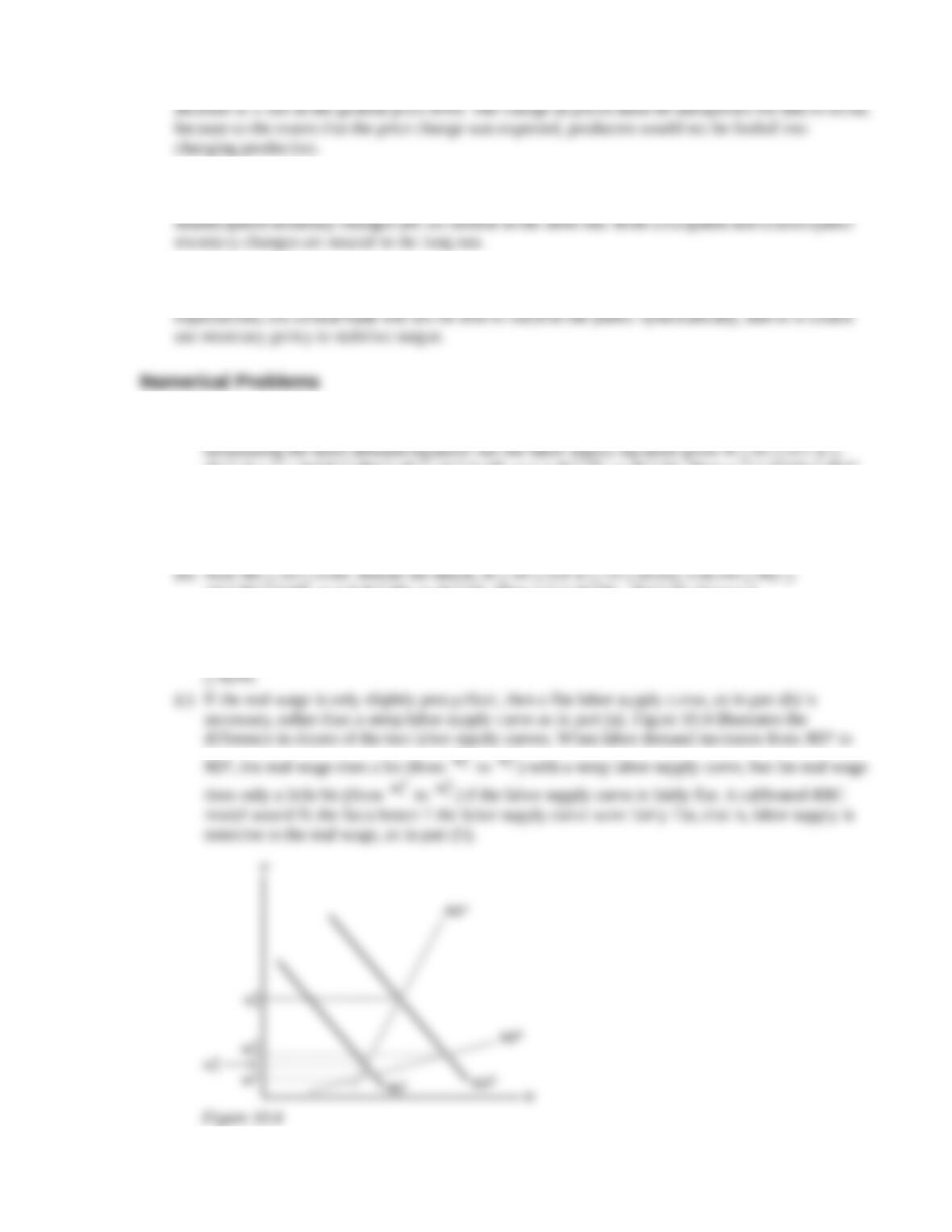
1. (a) Labor supply is given by the equation NS 45 0.1w. Before the shock, labor demand is
determined by the equation w 1.0(100 N). Setting labor supply equal to labor demand by
45 [0.1 1.0(100 N)] 45 10 0.1N, or 1.1 N 55, so N 50. Then w 1.0(100 N)
50. Output is Y 1.0[(100 50) (0.5 502)] 3750.
After the shock, repeating the above steps gives N 45 0.1 w 45 [0.1 1.1(100 N)]
45 11 0.11N, or 1.11 N 56, so N 50.45. Then w 1.1(100 N) 54.505. Output is
Y 1.1[(100 50.45) (0.5 50.452)] 4150.
10 80 0.8N, or 1.8 N 90, so N 50. Then w 1.0(100 – N) 50. Output is
Y 1.0[(100 50) (0.5 502)] 3750.
After the shock, N 10 0.8 w 10 [0.8 1.1(100 N)] 10 88 0.88N, or 1.88 N 98,
so N 52.13. Then w 1.1(100 N) 52.66. Output is Y 1.1[(100 52.13) (0.5 52.132)]
ND2, the real wage rises a lot (from
1
a
w
to
2
a
w
) with a steep labor supply curve, but the real wage
rises only a little bit (from
1
b
w
to
2
b
w
) if the labor supply curve is fairly flat. A calibrated RBC
model would fit the facts better if the labor supply curve were fairly flat, that is, labor supply is
sensitive to the real wage, as in part (b).
Figure 10.4

2. The IS curve gives Y C I G 600 0.5(Y T) 50r 450 50r G 1050 100r 0.5Y
0.5T G, or 0.5Y 1050 100r 0.5T G, or Y 2100 200r T 2G. The LM curve gives
M/P L 0.5Y 100i 0.5Y 100(r ) 0.5Y 100(r 0.05) 0.5Y 100r 5.
150) 2250 200r. Output must be at its full-employment level of 2210. From the IS curve,
2210 2250 200r, or 200r 40, so r 0.20. Using this in the LM curve to find the price level
gives M/P 0.5Y 100r 5, or 4320/P (0.5 2210) (100 0.20) 5, so P 4320/(1105
20 5) 4320/1080 4. Then consumption is C 600 0.5(Y T) – 50r 600 0.5(2210
150)
(50 0.20) 600 1030 10 1620. Investment is I 450 50r 450 (50 0.20) 440.
190 (2 190) 2290 200r. With Y 2210, this gives 2210 2290 200r, or 200r 80,
so r 0.40. From the LM curve, 4320/P 0.5Y 100r 5 (0.5 2210) (100 0.40) 5
1105 40 5 1060, so P 4320/1060 4.075. C 600 0.5(Y T) – 50r 600 0.5(2210
190) (50 0.40) 600 1010 20 1590. I 450 50r 450 (50 0.40) 430. Fiscal
3. The IS curve is found by setting desired saving equal to desired investment. Desired saving is
Sd Y Cd G Y [250 0.5(Y T) 500r] G. Setting Sd Id gives Y [250 0.5(Y T)
500r] G 250 500r, or Y 1000 2000r 2G T. The LM curve is M/P L 0.5Y 500i
0.5Y 500(r e) 0.5Y 500r.
(a) T G 200, M 7650. The IS curve gives Y 1000 2000r 2G T 1000 2000r
by 4 and rearrange the resulting equation and the IS curve.
LM: 7650/P 0.5Y 500r. Multiplying by 4 gives 30,600/P 2Y 2000r. Rearranging gives
2000r 2Y 30,600/P. IS: Y 1200 2000r. Rearranging gives 2000r 1200 Y. Setting the
right-hand sides of these two equations to each other (since both equal 2000r) gives: 2Y
(30,600/P) 1200 Y, or 3Y 1200 (30,600/P), or Y 400 (10,200/P); this is the AD curve.
With Y 1000 at full employment, the AD curve gives 1000 400 (10,200/P), or P 17.
From the IS curve Y 1200 2000r, so 1000 1200 2000r, or 2000r 200, so r 0.10.
4. AD: Y 300 30(M/P), AS: Y 500 10(P – Pe), M 400.
(a) Pe 60. Setting AD AS to eliminate Y, we get 300 30(M/P) 500 10(P Pe). Plugging in
10P 600, or 400 (12,000/P) 10P. Multiplying this equation through by P/10 gives 40P
1200 P2, or P2 40P 1200 0. This can be factored into (P 60)(P 20) 0. P can’t be
negative, so the only solution to this equation is P 60. At this equilibrium P Pe, so Y 500,
300 (21,000/P). The aggregate supply curve is Y 500 10(P Pe) 500 10(P 60) 10P
100. Setting AD AS to eliminate Y gives 300 (21,000/P) 10P 100, or 400 (21,000/P)
5. (a) To find the Solow residual, use the equation for the production function, dividing through to
solve for A: A Y/K0.3N0.7. Assuming there’s no change in utilization rates, this is the measured
Solow residual. Given that equation, plugging in the values for Y, K, and N, gives the Solow
residual as 1.435 in 2006 and 1.507 in 2007. The growth rate of the Solow residual is
in 2006 (as in part a), and 1.476 in 2007. This is an increase in productivity of [(1.476/1.435)
1] 100% 2.9%, significantly less than the 5.0% increase in the Solow residual.
(d) Setting uN 1 in year 2006 and 1.03 in year 2007, and uK 1 in year 2006 and 1.03 in year 2007,
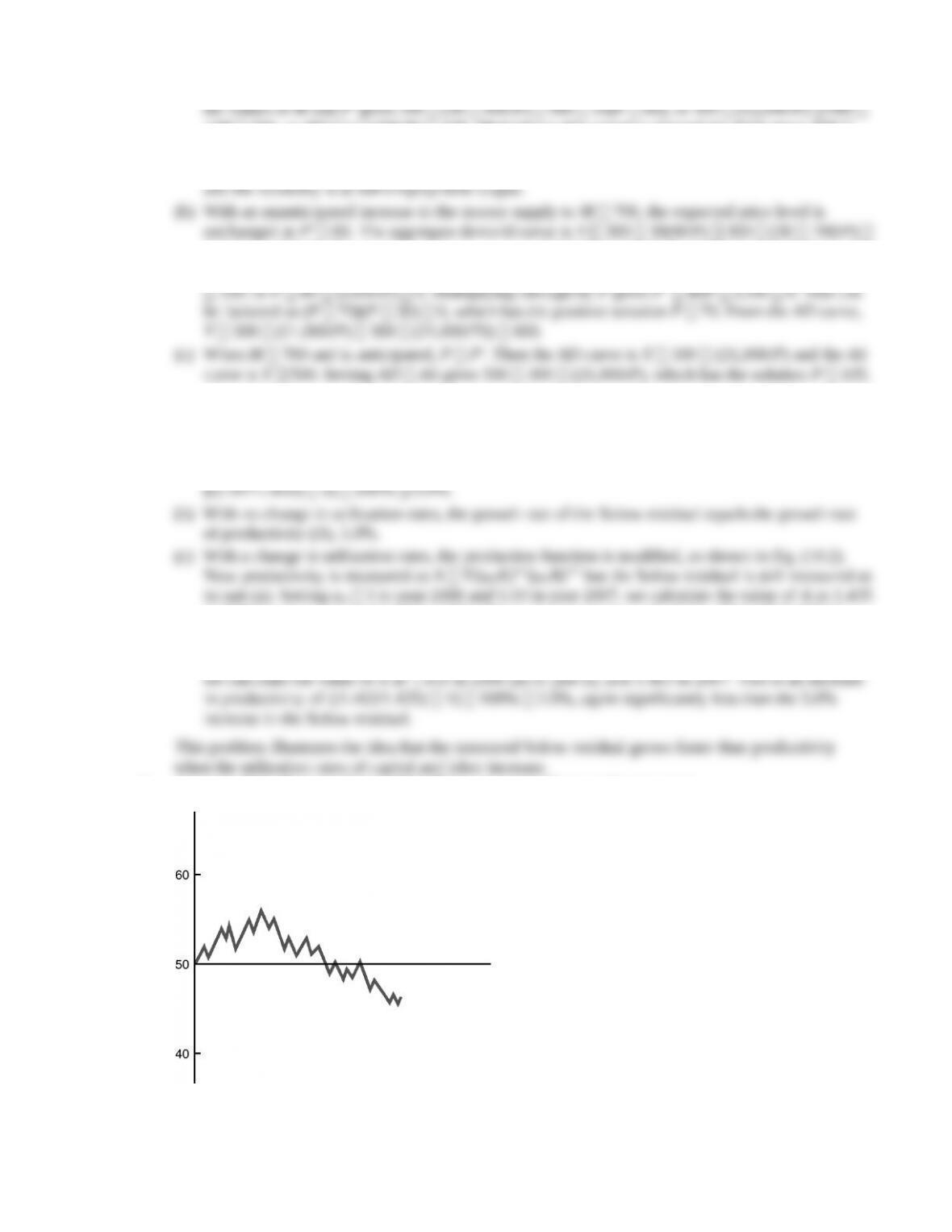
6. An example is shown in Figure 10.5. There are several long cycles in output.
Figure 10.5
7. (a) With an unemployment rate of 5%, there are initially 5 million unemployed and 95 million

employed. Since 1% of the employed become unemployed, 95 million 0.01 950,000 move
from employment to unemployment each month. Since 19% of the unemployed become
employed, 5 million 0.19 950,000 from unemployment each month. Since the same number
move from employed to unemployed as the number moving from unemployed to employed, the
8. (a) IS 2.47, IS 0.0004, LM 0, LM 0.001, lr 500, b 100.
(b) Y [2.47 88,950/(P 500)]/(.0004 .001) (2.47 177.9/P)/.0014
3085 100P (2.47 177.9/P)/.0014; multiply through by P and .0014 to get
4.319P .14P2 2.47P 177.9, or .14P2 1.849P 177.9 0; use quadratic formula:
P 29.65. Y 3085 100P 6050.
1. (a) The increase in MPKf leaves aggregate supply unchanged, since expected future labor income
and expected future wages are unchanged. But aggregate demand increases, because firms
increase investment, shifting the IS curve up and to the right. There is no shift in either the LM
curve or the FE line.
Figure 10.6(a) shows that the increase in aggregate demand causes no change in output, since the
2. (a) In the case of a permanent increase in government purchases, the income effect on labor supply,
which arises because the present value of taxes increases to pay for the added government
spending, is much higher than in the case of a temporary increase in government spending. So
workers increase their labor supply more when the government spending change is permanent
than when it is temporary.
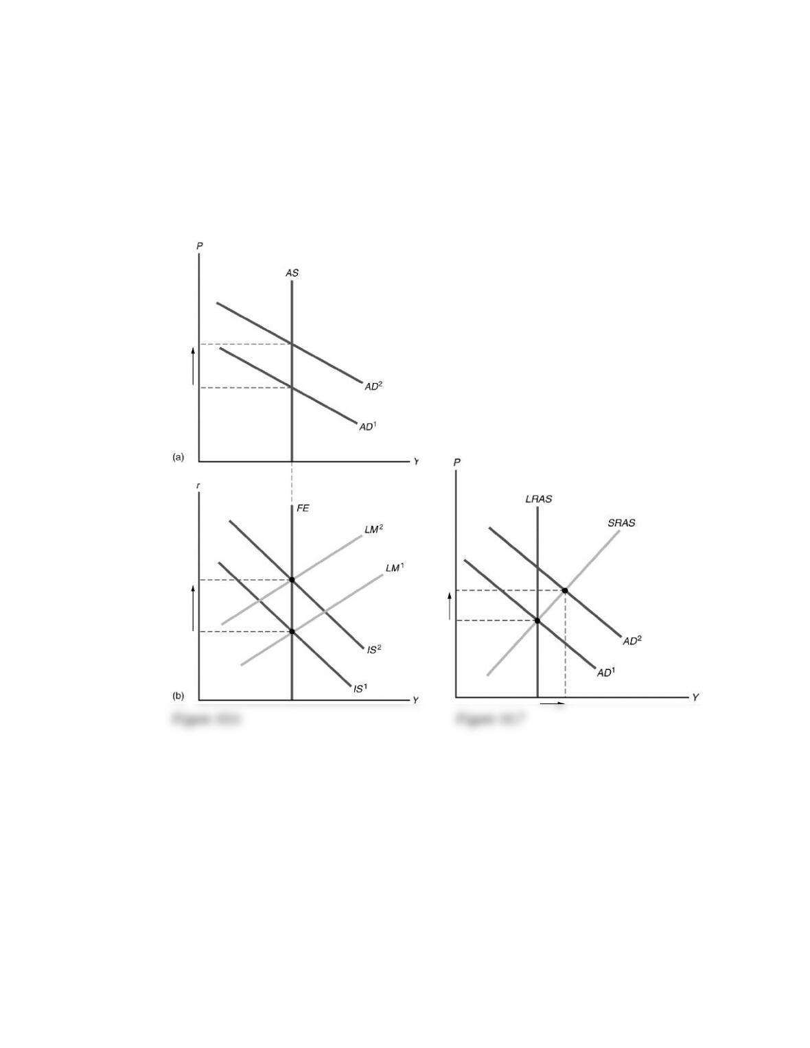
100, and in fact, the real interest rate and the price level may even rise if the IS curve shifts by a
lot, as shown in the figure.
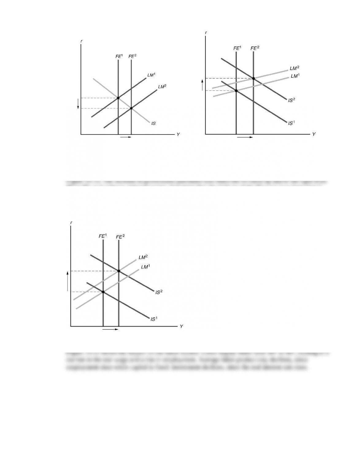
3. The temporary increase in government purchases causes an income effect that increases workers’
labor supply. This results in an increase in the full-employment level of output from FE1 to FE2 in
IS1 to IS2, as it reduces national saving. Assuming that the shift up of the IS curve is so large that it
intersects the LM curve to the right of the FE line, the price level must rise to get back to equilibrium
at full employment, by shifting the LM curve up and to the left from LM1 to LM2. The result is an
increase in output and the real interest rate.
Figure 10.10
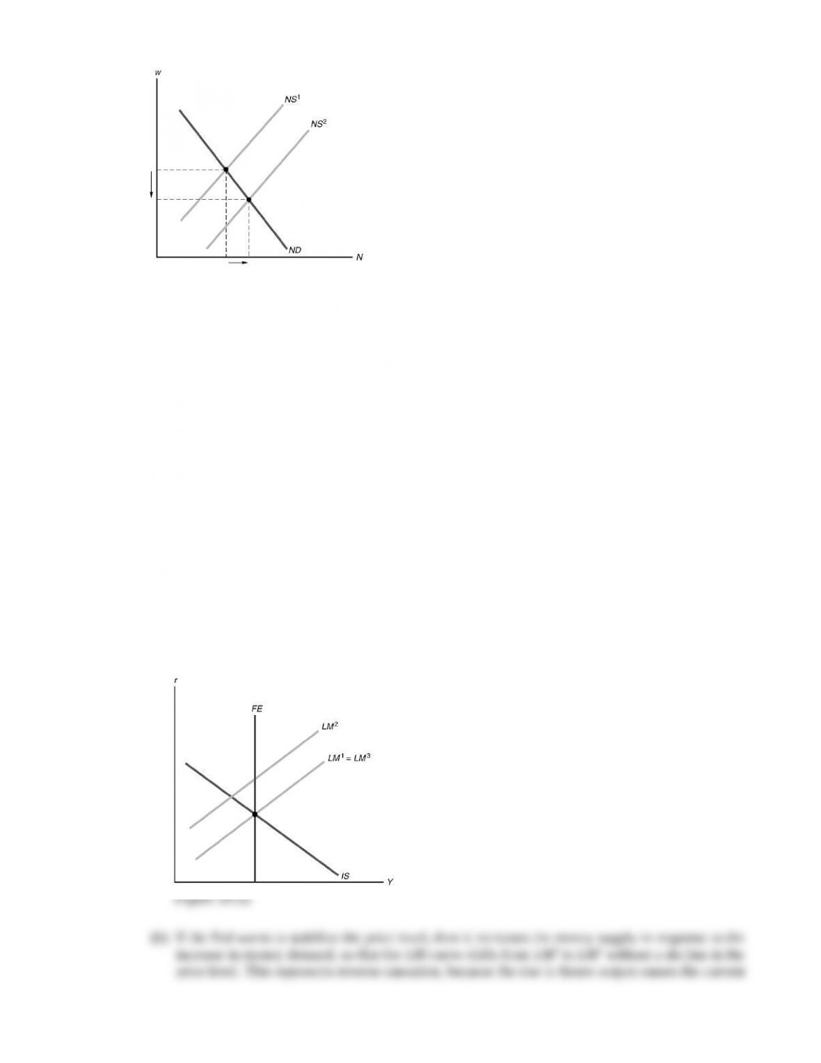
4.(a) An increase in expected future output increases money demand, so the LM curve shifts up and to the
left. As shown in Figure 10.12, the LM curve shifts from LM1 to LM2. General equilibrium in the
economy can be restored by shifting the LM curve from LM2 to LM3, which occurs as the price level
declines.
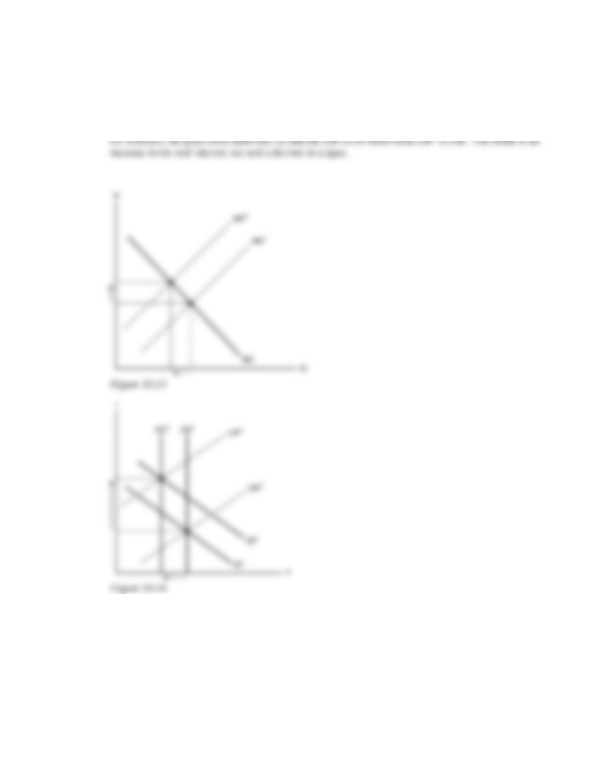
5. The temporary wage tax has a small income effect but a large substitution effect, so labor supply is
reduced. As Figure 10.13 shows, this increases the (pretax) real wage rate and reduces employment.
The reduction in employment shifts the FE line from FE1 to FE2 in Figure 10.14, while the increase
in government purchases shifts the IS curve from IS1 to IS2. To restore equilibrium, where IS, LM, and
1. The main feature of the classical IS-LM model that distinguishes it from the Keynesian IS-LM model
is the classical model’s assumption that prices adjust quickly to restore equilibrium. Keynesians
2. The two main components of any theory of the business cycle are (1) a specification of the types of
shocks or disturbances that are believed to be the most important in affecting the economy and (2) a
3. A real shock is a disturbance to the real side of the economy that affects the IS curve or the FE line.
A nominal shock is a disturbance to money supply or money demand that affects the LM curve. Real
shocks include changes in the production function, in the size of the labor force, in the real quantity
of government purchases, or in the spending and saving decisions of consumers. Real business cycle
4. RBC theory is successful at explaining that employment is procyclical, that average labor productivity
is procyclical, that the real wage is mildly procyclical, and that investment is more volatile than
5. The Solow residual is the most common measure of productivity shocks. It is strongly procyclical,
rising in expansions and declining in contractions. The Solow residual changes when total factor
6. The increase in government purchases does not affect labor demand, but causes an increase in labor
supply at any given real wage. This occurs because workers are poorer due to the current or future
taxes they must pay to finance the increased government spending. Since labor demand is unchanged
but labor supply increases, the real wage declines and employment rises. The rise in employment
7. Reverse causation means that expected future increases in output cause increases in the current
money supply, and expected future decreases in output cause decreases in the current money supply.
8. According to the misperceptions theory, an increase in the price level fools producers of goods into
producing more, because they are unable to tell whether the increase in prices is a relative price
9. In the classical model, money is neutral in both the short run and the long run. This is modified in the
misperceptions theory in that anticipated monetary changes are neutral in the short run, but
10. Rational expectations means that the public’s forecasts of various economic variables are based on
reasoned and intelligent examination of available economic data. If the public has rational
1. (a) Labor supply is given by the equation NS 45 0.1w. Before the shock, labor demand is
determined by the equation w 1.0(100 N). Setting labor supply equal to labor demand by
45 [0.1 1.0(100 N)] 45 10 0.1N, or 1.1 N 55, so N 50. Then w 1.0(100 N)
50. Output is Y 1.0[(100 50) (0.5 502)] 3750.
After the shock, repeating the above steps gives N 45 0.1 w 45 [0.1 1.1(100 N)]
45 11 0.11N, or 1.11 N 56, so N 50.45. Then w 1.1(100 N) 54.505. Output is
Y 1.1[(100 50.45) (0.5 50.452)] 4150.
10 80 0.8N, or 1.8 N 90, so N 50. Then w 1.0(100 – N) 50. Output is
Y 1.0[(100 50) (0.5 502)] 3750.
After the shock, N 10 0.8 w 10 [0.8 1.1(100 N)] 10 88 0.88N, or 1.88 N 98,
so N 52.13. Then w 1.1(100 N) 52.66. Output is Y 1.1[(100 52.13) (0.5 52.132)]
ND2, the real wage rises a lot (from
1
a
w
to
2
a
w
) with a steep labor supply curve, but the real wage
rises only a little bit (from
1
b
w
to
2
b
w
) if the labor supply curve is fairly flat. A calibrated RBC
model would fit the facts better if the labor supply curve were fairly flat, that is, labor supply is
sensitive to the real wage, as in part (b).
Figure 10.4
2. The IS curve gives Y C I G 600 0.5(Y T) 50r 450 50r G 1050 100r 0.5Y
0.5T G, or 0.5Y 1050 100r 0.5T G, or Y 2100 200r T 2G. The LM curve gives
M/P L 0.5Y 100i 0.5Y 100(r ) 0.5Y 100(r 0.05) 0.5Y 100r 5.
150) 2250 200r. Output must be at its full-employment level of 2210. From the IS curve,
2210 2250 200r, or 200r 40, so r 0.20. Using this in the LM curve to find the price level
gives M/P 0.5Y 100r 5, or 4320/P (0.5 2210) (100 0.20) 5, so P 4320/(1105
20 5) 4320/1080 4. Then consumption is C 600 0.5(Y T) – 50r 600 0.5(2210
150)
(50 0.20) 600 1030 10 1620. Investment is I 450 50r 450 (50 0.20) 440.
190 (2 190) 2290 200r. With Y 2210, this gives 2210 2290 200r, or 200r 80,
so r 0.40. From the LM curve, 4320/P 0.5Y 100r 5 (0.5 2210) (100 0.40) 5
1105 40 5 1060, so P 4320/1060 4.075. C 600 0.5(Y T) – 50r 600 0.5(2210
190) (50 0.40) 600 1010 20 1590. I 450 50r 450 (50 0.40) 430. Fiscal
3. The IS curve is found by setting desired saving equal to desired investment. Desired saving is
Sd Y Cd G Y [250 0.5(Y T) 500r] G. Setting Sd Id gives Y [250 0.5(Y T)
500r] G 250 500r, or Y 1000 2000r 2G T. The LM curve is M/P L 0.5Y 500i
0.5Y 500(r e) 0.5Y 500r.
(a) T G 200, M 7650. The IS curve gives Y 1000 2000r 2G T 1000 2000r
by 4 and rearrange the resulting equation and the IS curve.
LM: 7650/P 0.5Y 500r. Multiplying by 4 gives 30,600/P 2Y 2000r. Rearranging gives
2000r 2Y 30,600/P. IS: Y 1200 2000r. Rearranging gives 2000r 1200 Y. Setting the
right-hand sides of these two equations to each other (since both equal 2000r) gives: 2Y
(30,600/P) 1200 Y, or 3Y 1200 (30,600/P), or Y 400 (10,200/P); this is the AD curve.
With Y 1000 at full employment, the AD curve gives 1000 400 (10,200/P), or P 17.
From the IS curve Y 1200 2000r, so 1000 1200 2000r, or 2000r 200, so r 0.10.
4. AD: Y 300 30(M/P), AS: Y 500 10(P – Pe), M 400.
(a) Pe 60. Setting AD AS to eliminate Y, we get 300 30(M/P) 500 10(P Pe). Plugging in
10P 600, or 400 (12,000/P) 10P. Multiplying this equation through by P/10 gives 40P
1200 P2, or P2 40P 1200 0. This can be factored into (P 60)(P 20) 0. P can’t be
negative, so the only solution to this equation is P 60. At this equilibrium P Pe, so Y 500,
300 (21,000/P). The aggregate supply curve is Y 500 10(P Pe) 500 10(P 60) 10P
100. Setting AD AS to eliminate Y gives 300 (21,000/P) 10P 100, or 400 (21,000/P)
5. (a) To find the Solow residual, use the equation for the production function, dividing through to
solve for A: A Y/K0.3N0.7. Assuming there’s no change in utilization rates, this is the measured
Solow residual. Given that equation, plugging in the values for Y, K, and N, gives the Solow
residual as 1.435 in 2006 and 1.507 in 2007. The growth rate of the Solow residual is
in 2006 (as in part a), and 1.476 in 2007. This is an increase in productivity of [(1.476/1.435)
1] 100% 2.9%, significantly less than the 5.0% increase in the Solow residual.
(d) Setting uN 1 in year 2006 and 1.03 in year 2007, and uK 1 in year 2006 and 1.03 in year 2007,
6. An example is shown in Figure 10.5. There are several long cycles in output.
Figure 10.5
7. (a) With an unemployment rate of 5%, there are initially 5 million unemployed and 95 million
employed. Since 1% of the employed become unemployed, 95 million 0.01 950,000 move
from employment to unemployment each month. Since 19% of the unemployed become
employed, 5 million 0.19 950,000 from unemployment each month. Since the same number
move from employed to unemployed as the number moving from unemployed to employed, the
8. (a) IS 2.47, IS 0.0004, LM 0, LM 0.001, lr 500, b 100.
(b) Y [2.47 88,950/(P 500)]/(.0004 .001) (2.47 177.9/P)/.0014
3085 100P (2.47 177.9/P)/.0014; multiply through by P and .0014 to get
4.319P .14P2 2.47P 177.9, or .14P2 1.849P 177.9 0; use quadratic formula:
P 29.65. Y 3085 100P 6050.
1. (a) The increase in MPKf leaves aggregate supply unchanged, since expected future labor income
and expected future wages are unchanged. But aggregate demand increases, because firms
increase investment, shifting the IS curve up and to the right. There is no shift in either the LM
curve or the FE line.
Figure 10.6(a) shows that the increase in aggregate demand causes no change in output, since the
2. (a) In the case of a permanent increase in government purchases, the income effect on labor supply,
which arises because the present value of taxes increases to pay for the added government
spending, is much higher than in the case of a temporary increase in government spending. So
workers increase their labor supply more when the government spending change is permanent
than when it is temporary.
100, and in fact, the real interest rate and the price level may even rise if the IS curve shifts by a
lot, as shown in the figure.
3. The temporary increase in government purchases causes an income effect that increases workers’
labor supply. This results in an increase in the full-employment level of output from FE1 to FE2 in
IS1 to IS2, as it reduces national saving. Assuming that the shift up of the IS curve is so large that it
intersects the LM curve to the right of the FE line, the price level must rise to get back to equilibrium
at full employment, by shifting the LM curve up and to the left from LM1 to LM2. The result is an
increase in output and the real interest rate.
Figure 10.10
4.(a) An increase in expected future output increases money demand, so the LM curve shifts up and to the
left. As shown in Figure 10.12, the LM curve shifts from LM1 to LM2. General equilibrium in the
economy can be restored by shifting the LM curve from LM2 to LM3, which occurs as the price level
declines.
5. The temporary wage tax has a small income effect but a large substitution effect, so labor supply is
reduced. As Figure 10.13 shows, this increases the (pretax) real wage rate and reduces employment.
The reduction in employment shifts the FE line from FE1 to FE2 in Figure 10.14, while the increase
in government purchases shifts the IS curve from IS1 to IS2. To restore equilibrium, where IS, LM, and