Scott, Financial Accounting Theory, 7th Edition Instructor’s Solutions Manual Chapter 3
88
Copyright © 2015 Pearson Canada Inc.
A M Probabilities
High High (0.15 – 0.0850) × (0.10 – 0.0850) × 0.72 = 0.0007
High Low (0.15 – 0.0850) × (0.0250 – 0.0850) × 0.02 = –0.0001
Low High (-0.10 – 0.0850 × (0.10 – =0.0850 × 0.08 = –0.0002
Low Low (-0.10 – 0.0850) × (0.0250 – 0.0850) × 0.18) = 0.0020
Cov(A,M) = 0.0024
In the first row of the table, the values 0.15 and 0.0850 are the high return and the
expected return respectively of A (see Table 3.3). Similarly 0.10 and 0.0850 are the high
return and the expected return of M (see Section 3.6). The joint probability that both A
and M pay off high is:
Prob(A high and M high) = Prob(M high) Prob(A high|M high)
= 0.8 x 0.9
= 0.72
You should verify the remaining rows in the table.
Then, recalling from Section 3.6 that σ2M = Var(M) = 0.0009, we obtain:
𝛽𝐴=0.0024
0.0009 = 2.6667
For security B in Example 3.3, assume that the conditional payoff probabilities are:
■ When return on M is high:
Probability that return on B is high = 0.7917
Probability that return on B is low = 0.2083
■ When return on M is low:

Scott, Financial Accounting Theory, 7th Edition Instructor’s Solutions Manual Chapter 3
89
Probability that return on B is high = 0.2083
Probability that return on B is low = 0.7917
Then, similar calculations give:
𝛽𝐵=0.0014
0.0009 = 1.5556
You should verify this calculation.4
Since βB is lower than βA, an investor who buys only B shares is more insulated from
the ups and downs of the stock market than if he/she buys only A shares. This is the
sense in which a low–beta security has low risk.5
3.7.4 Summary
If we ignore the transactions costs of buying securities, the optimal investment decision
is to buy all securities available on the market, thereby obtaining maximum
diversification. The risk–averse investor’s desired risk/return trade–off can then be
attained by borrowing to buy the risk free asset, which increases expected return and
risk to the desired level. Conversely, risk can be reduced by selling a portion of the
market portfolio and investing the proceeds in the risk free asset.
When transactions costs are not ignored, this policy would be too costly. Then, the risk–
averse investor’s optimal investment decision is to buy fewer securities, rather than the
whole market portfolio. In this way, some of the benefits of diversification can be
attained, at reasonable cost. Information about securities’ expected returns and betas is
useful to such investors. This enables them to assess the expected return and riskiness
of various portfolios that they may be considering. They can then choose the portfolio
that gives them their most preferred risk–return trade–off, subject to the level of
transactions costs that they are willing to bear.
Notes

90
1. We have suppressed the set of states of nature in this example. That is, Toni
assesses payoff probabilities directly, rather than routing them through states. Thus,
instead of saying “The probability that firm A is in high–performance state is 0.74 and if
A really is in this state the payoff will be $230,” we simply say “The probability of the
$230 payoff is 0.74.” This simplification has certain analytical advantages and is
frequently used.
2. This argument assumes that the only source of correlation between returns on
firms’ shares is market–wide factors. In effect, we have partitioned states of nature that
can affect share returns into two components—economy–wide and firm–specific. This is
a simplification, since, for example, industry–wide factors could introduce additional
returns correlation. However, the simplification is a widely used one and is sufficient for
our purposes. It leads to an important measure of share riskiness (beta), which we will
discuss shortly.
3. The risk we are referring to here is ex ante risk. That is, the investor is in the
process of an investment decision and is looking ahead. This is not to say that if a firm
in the portfolio realizes, say, a low return because some unfortunate firm–specific risk
factor has happened, the investor will not be angry at that firm ex post.
4. The expected return of B is
�0.6750 ×92−80
60 �+�0.3250 ×76−80
80 �
= (0.6750 × 0.15) + (0.3250 × 20.05) = 0.0850
(See Example 3.3.)
Cov(B,M) is calculated as
Returns Joint Probabilities
B M
High High (0.15 – 0.085) × (0.10 – 0.085) × 0.6333 = 0.0006
High Low (0.15 – 0.085) × (0.025 – 0.085) × 0.0417 = 0.0002

Scott, Financial Accounting Theory, 7th Edition Instructor’s Solutions Manual Chapter 3
91
Low High (–0.05 – 0.085) × (0.10 – 0.085) × 0.1667 = 0.0003
Low Low (–0.05 – 0.085 × (0.025 – 0.085) × 0.1583 = 0.0013
Cov(B,M) = 0.0014
The joint probability of B high and M high is given by 0.8 × 0.7917 = 0.6333. You should
now verify the remaining lines.
5. Note that A shares have the same expected return as B shares (0.085), but
higher risk since βA = 2.6667 while βB = 1.5556. Then, it might seem that Toni should
buy only B shares. However, this is not the case—Toni will still want to hold both A and
B shares in her portfolio. If she invests all of her $200 in B, it can be shown that her
expected return is 0.085 and variance of return is 0.0088, giving expected utility of
0.1612, which is less than expected utility of 0.1626 from holding both A and B. In this
case, the benefits of diversification outweigh the fact that B shares by themselves have
lower risk.
6. MD&A
I feel it is important to bring the students back to some specific financial reporting issues
to show how accountants are grappling with the full disclosure implications of decision
usefulness, particularly reporting on firm risk. For this purpose, I use MD&A.
I usually hand out an example of at least the risks and uncertainties and future–oriented
sections of MD&A from a current annual report, or ask the students to choose an annual
report, and assign a critique of its MD&A disclosure, using the example in the chapter
as a template. Discussion of the information content of the MD&A often reveals a
tendency for firms to rehash information already available from other parts of the annual
report, and to give only vague discussion, if any, of risks and uncertainties and future
plans. I ask why some firms choose to give extensive and candid disclosure.
Favourable impacts on cost of capital (see the discussion in Section 12.9) and even on
product markets are possibilities.
In this edition, I have added a section (Section 3.6.4) on the decision usefulness of
MD&A. This research is relatively new. Coverage of this section is not essential.

Scott, Financial Accounting Theory, 7th Edition Instructor’s Solutions Manual Chapter 3
92
However, it may be of interest to students and instructors who wish to consider how
sophisticated programs to evaluate the written word can be applied to a topic of interest
to accountants. The study of Li (2010) can also be used to show an application of
Bayesian decision theory considered in this chapter. In Theory in Practice 3.3 I have
organized my outline of Li’s study to be consistent with the earlier decision theory
development, particularly in how the information system can be derived. The study of
Brown and Tucker (2011) is more straightforward.
6. The Conceptual Framework
As a final step in motivating the decision theory, I outline Chapters 1 and 3 of the
Conceptual Framework. In particular, I show how the theory shows up in the
Framework, by discussing how it has “bought” the decision usefulness approach.
The main difference from the decision theory model presented in the text is that the
word ‘rational” does not appear as a specific investor characteristic. Possibly, this is
because of the theory and evidence from behavioural finance that disputes rationality
(although I have been told in correspondence by a member of the IASB at the time that
it is hard to envisage non–rational decision making). Also, the Framework envisages the
role of financial reporting as providing information to a wide variety of constituencies,
not just to investors. Since “true” net income does not exist, and since different users
have decision needs, it is not clear to me how a single set of financial statements can
cater to different user constituencies. Nevertheless, the role of financial reporting as
conveying useful information to decision makers comes through clearly in the
Framework.
The word “rational” was used in SFAC 1, being Chapter 1 of the original FASB
conceptual framework. Some instructors may be interested in the route by which such
an abstract theory as the theory of rational decision entered into the FASB concepts
statements. The source appears to be the American Institute of Certified Public
Accountants Study Group on the Objectives of Financial Statements, “Objectives of
Financial Statements,” (New York, NY: AICPA, 1973), also known as the Trueblood

Scott, Financial Accounting Theory, 7th Edition Instructor’s Solutions Manual Chapter 3
93
Report. According to Zeff in his article “The Evolution of the Conceptual Framework for
Business Enterprises in The United States,” (Accounting Historians Journal (December,
1999)), the Trueblood Report provided a “blueprint” for the FASB concepts statements.
This can be seen with particular clarity in Volume 2: Selected Papers of the Trueblood
Report, which contains several studies on the use of accounting information in
normative models of investor consumption/investment decisions. See, in particular,
Ronen, J., “A User Oriented Development of Accounting Information
Requirements,” in J. J. Cramer and G. H. Sorter, editors., Objectives of
Financial Statements: Volume 2 / Selected Papers (The Trueblood
Report) (New York, NY: American Institute of Certified Public Accountants,
1974), pp. 80–103.
Ronen, J. and G. H. Sorter, “The Descriptive and the Normative,” in J. J.
Cramer and G. H. Sorter, editors., Objectives of Financial Statements:
Volume 2 / Selected Papers (The Trueblood Report) (New York, NY:
American Institute of Certified Public Accountants, 1974), pp. 24–29.

Scott, Financial Accounting Theory, 7th Edition Instructor’s Solutions Manual Chapter 3
94
SUGGESTED SOLUTIONS TO QUESTIONS AND PROBLEMS
1. Perfect or Fully–Informative Information System
Current Financial Statement Information
Prior probabilities of the states of nature are:
(any other set of prior probabilities with P(H) > 0 would do)
Suppose that GN is observed. Then, by Bayes’ theorem:
00.1
)070.0()00.130.0(
00.130.0
)/()()/()(
)/()(
)/(
=
×+×
×
=
+
=LGHPLPHGNPHP
HGNPHP
GNHP

Scott, Financial Accounting Theory, 7th Edition Instructor’s Solutions Manual Chapter 3
95
0
)070.0()00.130.0(
070.0
)/()()/()(
)/()(
)/(
=
×+×
×
=
+
=LGNPLPHGNPHP
LGNPLP
GNLP
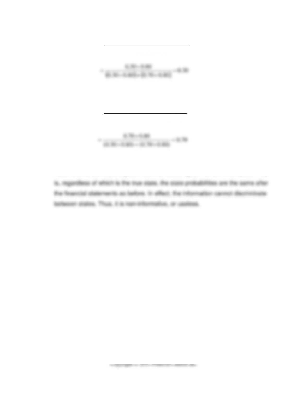
Thus, with a perfect information system, the information perfectly reveals the true
state of nature.
Non–Informative Information System
Current Financial Statement Information
GN BN
Here, both rows of the information system are the same. Any system with both
row probabilities the same would do.
Note: Students have a tendency to use 0.5 probability in each row. This is OK,
Suppose that GN is observed. Then, by Bayes’ theorem:
Scott, Financial Accounting Theory, 7th Edition Instructor’s Solutions Manual Chapter 3
)/()()/()(
)/()(
)/(
+
=LGNPLPHGNPHP
HGNPHP
GNHP
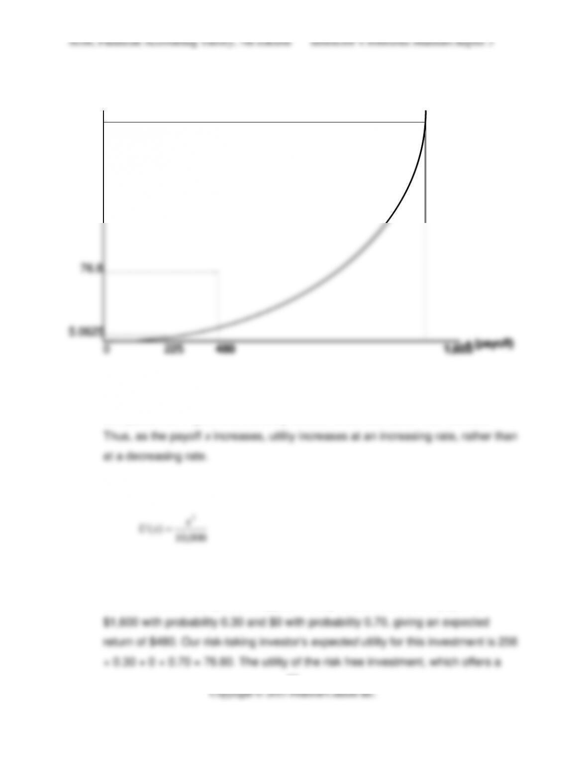
2. The utility function of a risk–taking investor would appear as the solid line below:
Compared with Figure 3.3, the utility function is convex, rather than concave.
A specific example of a risk–taking utility function is:
000,10
)(
2
x
xU =
yielding the utilities shown on the vertical axis of the above figure.
Consistent with Example 3.1, suppose a risky investment offers a payoff of
U(x)
256
76.8
5.0625
0 225 480 1,600
x (payoff)
U(x)
256
76.8
5.0625
0 225 480 1,600
x (payoff)

Scott, Financial Accounting Theory, 7th Edition Instructor’s Solutions Manual Chapter 3
98
payoff of $225 for sure, is only 5.0625. Thus, for the same prior probabilities and
A risk–taking investor will specialize (that is, buy only one security) — the one
A risk–taking investor needs the same information as any other investor —
3. For a2 to yield the same utility as a1, we must have:
384.22/180.03
384.22/13
2
2
2
=−×
=−
x
xa
x
σ
σ
Solving for
2
x
σ
:
384.2400.22/1
2
−=
x
σ
A risk–averse investor trades off risk and expected return. An investment act with

Scott, Financial Accounting Theory, 7th Edition Instructor’s Solutions Manual Chapter 3
100
4. The argument is probably made because of the “lumpiness” of certain cash
receipts and disbursements. Cash payments for major purchases such as capital
assets, and for borrowings such as loan proceeds, tend to occur at discrete
intervals in large amounts. As a result, a firm could have what appears as a

103
8. a. Mr. Smart derives the following utilities from the payoffs:
2ln(8,000) = 17.97
Based on his prior probabilities, Mr. Smart has the following expected utilities for
the two actions:
Thus, to maximize expected utility, Mr. Smart should buy the mutual fund.
b. Let:
G = good state of the economy
B = bad state of the economy
S = evidence obtained from financial statements
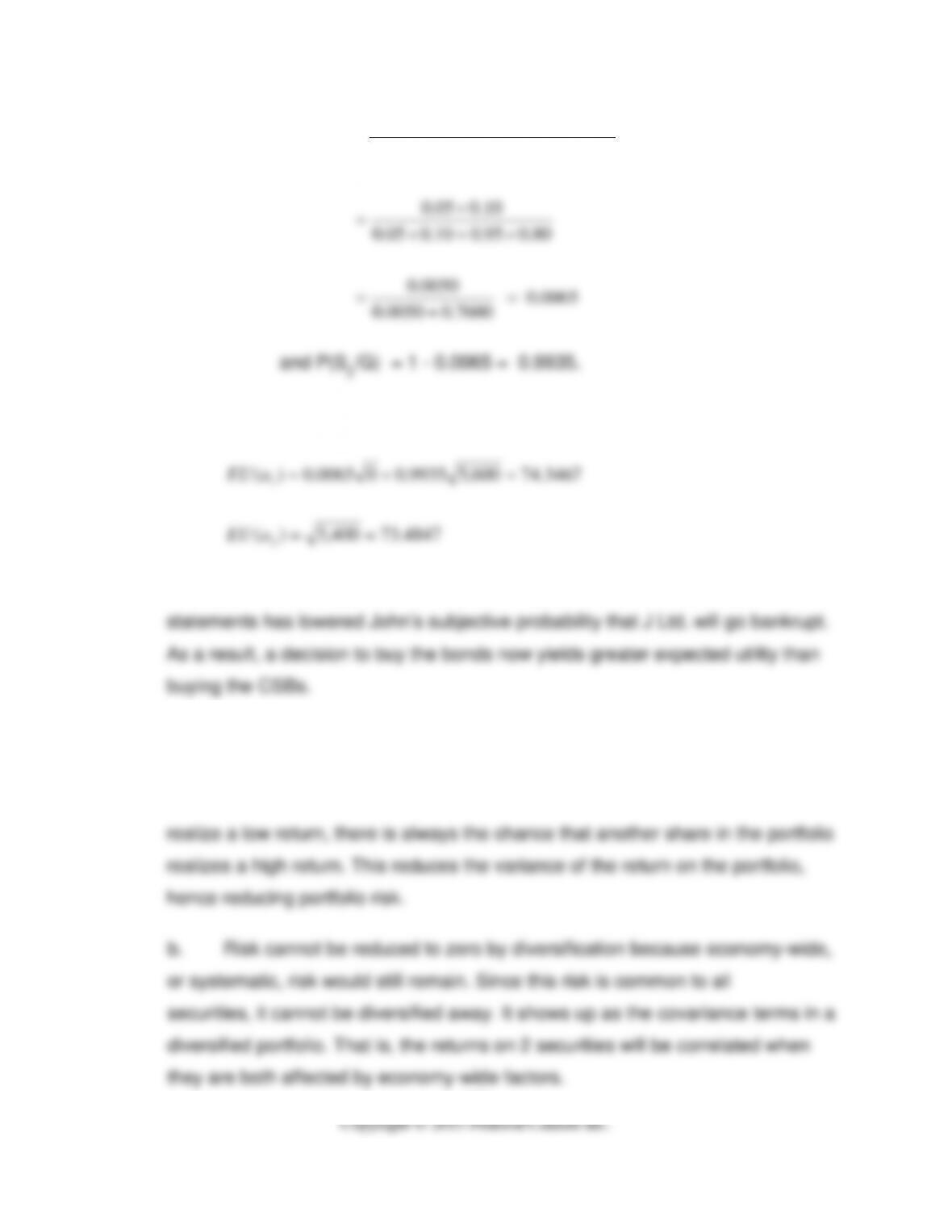
Then, by Bayes’ theorem, the posterior probability of the good state is:

Scott, Financial Accounting Theory, 7th Edition Instructor’s Solutions Manual Chapter 3
)/()()/()(
)/()(
)/(
+
=BSPBPGSPGP
GSPGP
SGP
Scott, Financial Accounting Theory, 7th Edition Instructor’s Solutions Manual Chapter 3
10.005.0
)/()()/()(
)/()(
)/(
2211
11
1
×
+
=SGPSPSGPSP
SGPSP
GSP

106
11. a. The payoff table for Marie’s decision is:
Act State
Not Bankrupt Bankrupt
Based on her prior probabilities and square root utility function, the expected
utility of each act is:
04.0144,16.0)( 1×+×=aEU
Therefore, Marie should take a2 and buy the CSB.
Note: Payoffs are evaluated gross in this question since negative payoffs are not
defined for square root utility.
b. From Bayes’ theorem, Marie’s posterior probabilities over the states are:
30.0
5.06.0
×
The expected utility of each act now is: