Unlock document.
This document is partially blurred.
Unlock all pages and 1 million more documents.
Get Access
BUSINESS ANALYTICS MODULE B LI N EA R PR O G R A M M I N G 287
12
*
12
12
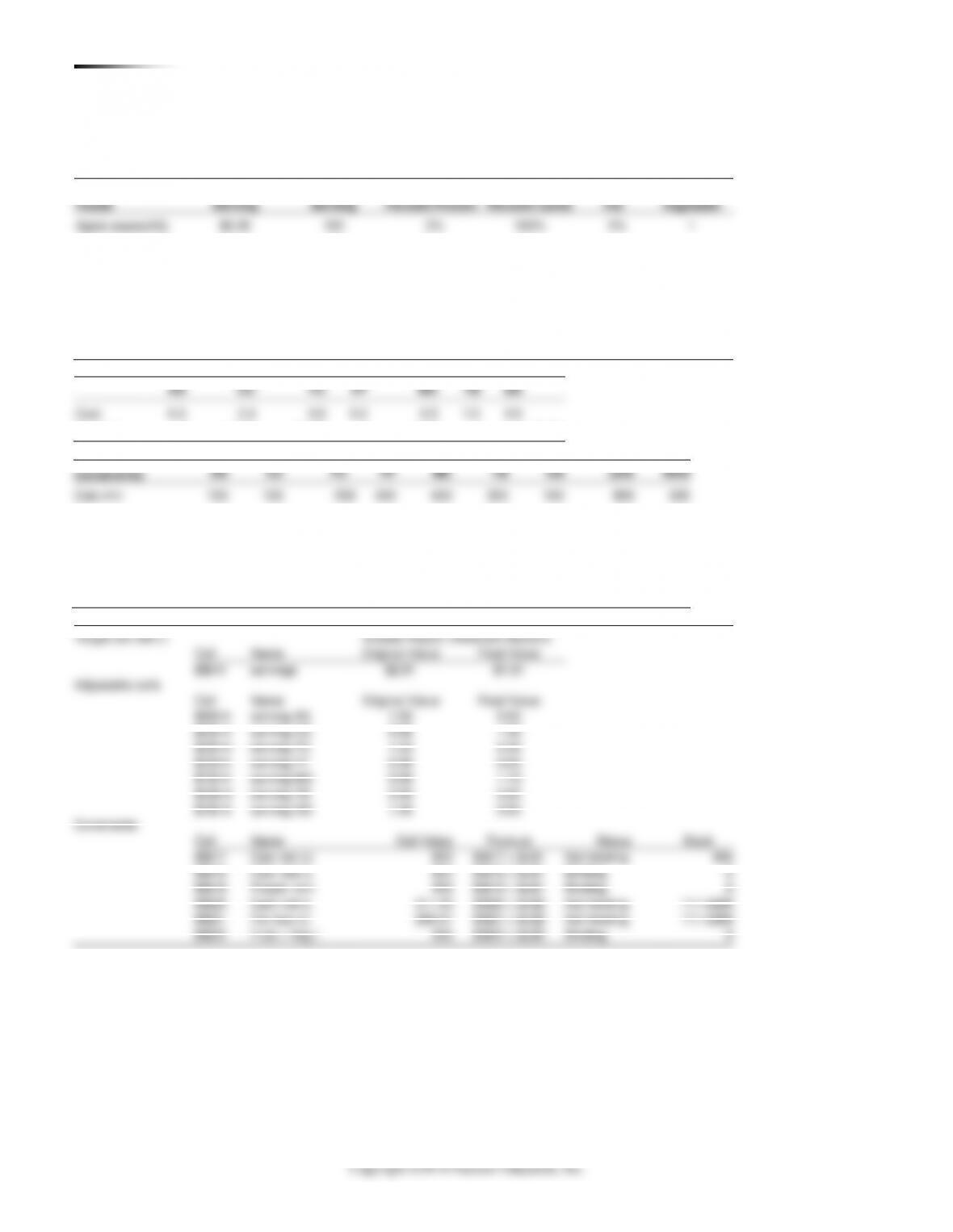
@ : ( 0, 100) Obj 9 0 20 100 $2,000.00
@ : ( 262.5, 25) Obj 9 262.5 20 25 $2,862.50
@ : ( 300, 0) Obj 9 300 20 0 $2,700.00
a x x
b x x
c x x
= = = + =
= = = + =
= = = + =
ADDITIONAL HOMEWORK PROBLEMS
Here are the answers to additional homework problems
B.31–B.40 that appear on our Web sites, www.myomlab.com and
at www.pearsonhighered.com/heizer.
B.31 Let x = number of standard model to produce
y = number of deluxe model to produce
Maximize 40x + 60y
Subject to 30 30 450
10 15 180
6
xy
xy
x
+
+
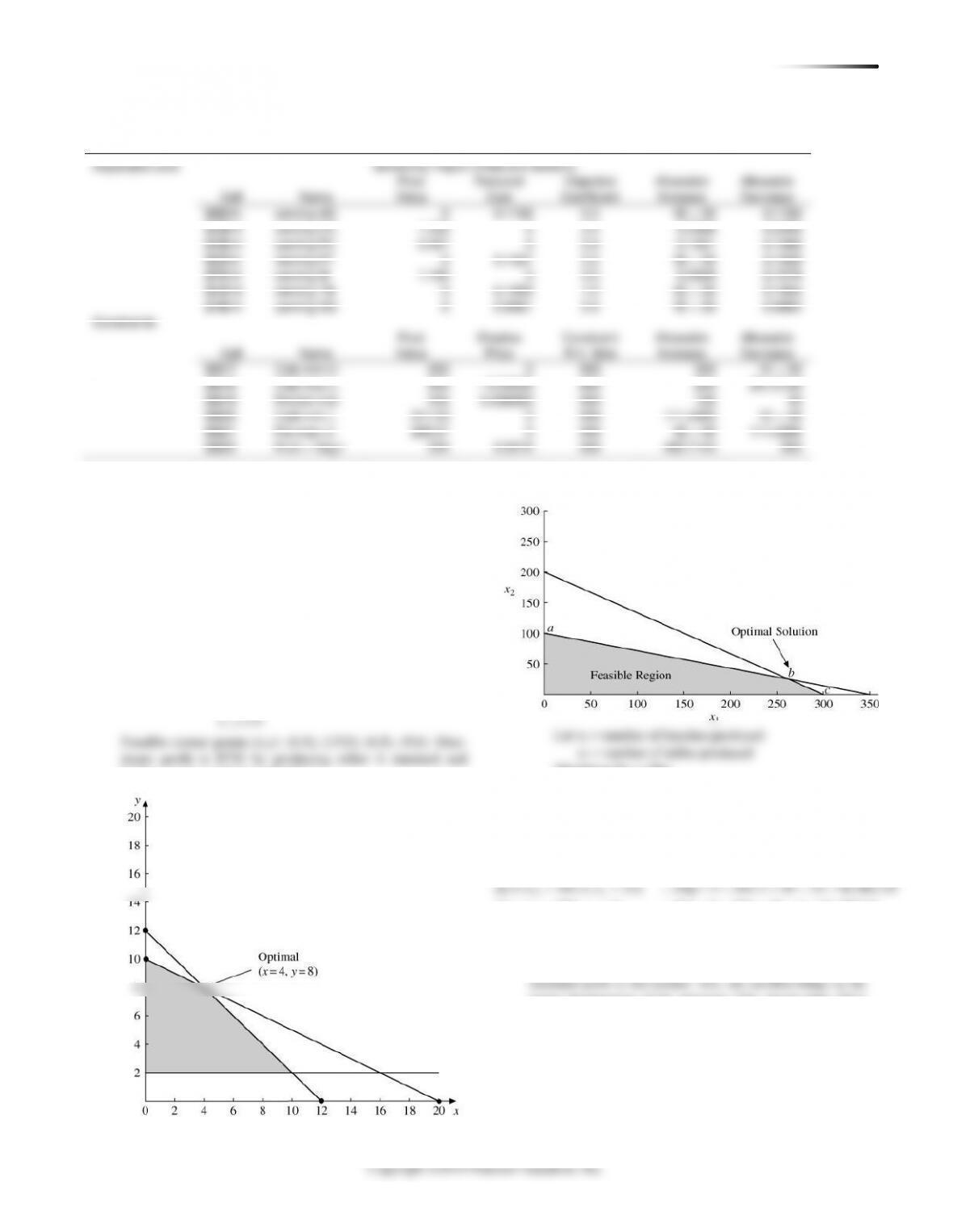
Feasible corner points (x,y): (6,0), (15,0), (6,8), (9,6). Max-
imum profit is $720 by producing either 6 standard and
8 deluxe or 9 standard and 6 deluxe.
B.33
x2 = number of tables produced
Maximize 9x1 + 20x2
Subject to 4x1 + 6x2 1,200 (hours)
10x1 + 35x2 3,500 (board-feet)
x1, x2 0 (non-negativity)
Profit:
Adjustable cells
Sensitivity Report (Relevant Section)
Cell
Name
Final
Value
Reduced
Cost
Objective
Coefficient
Allowable
Increase
Allowable
Decrease
$B$14
serving AS
0
0.1726
0.3
1E + 30
0.1726
$C$14
serving CC
1.333
0
0.4
0.2589
0.2256
$D$14
serving FC
0.457
0
0.9
0.1051
0.1006
$E$14
serving FF
0
0.1527
0.2
1E + 30
0.1529
$F$14
serving M
1.130
0
0.5
0.0629
0.7078
$G$14
serving TB
0
0.1693
1.5
1E + 30
0.1694
$H$14
serving GS
0
0.6661
0.9
1E + 30
0.6882
Constraints
Cell
Name
Final
Value
Shadow
Price
Constraint
R.H. Side
Allowable
Increase
Allowable
Decrease
$I$17
Cals min LI
800
0
500
300
1E + 30
$I$18
Cals max L
800
– 0.00023
800
200
251.6129
$I$19
Protein min
200
0.008983
200
155
40
$I$20
Carb min L
311.43
0
200
111.4285
1E + 30
$I$21
Fat max LI
288.57
0
400
1E + 30
111.4286
$I$22
Fruit + Veg I
200
0.0015
200
485.7143
200
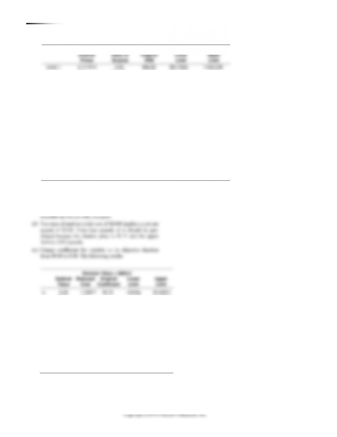
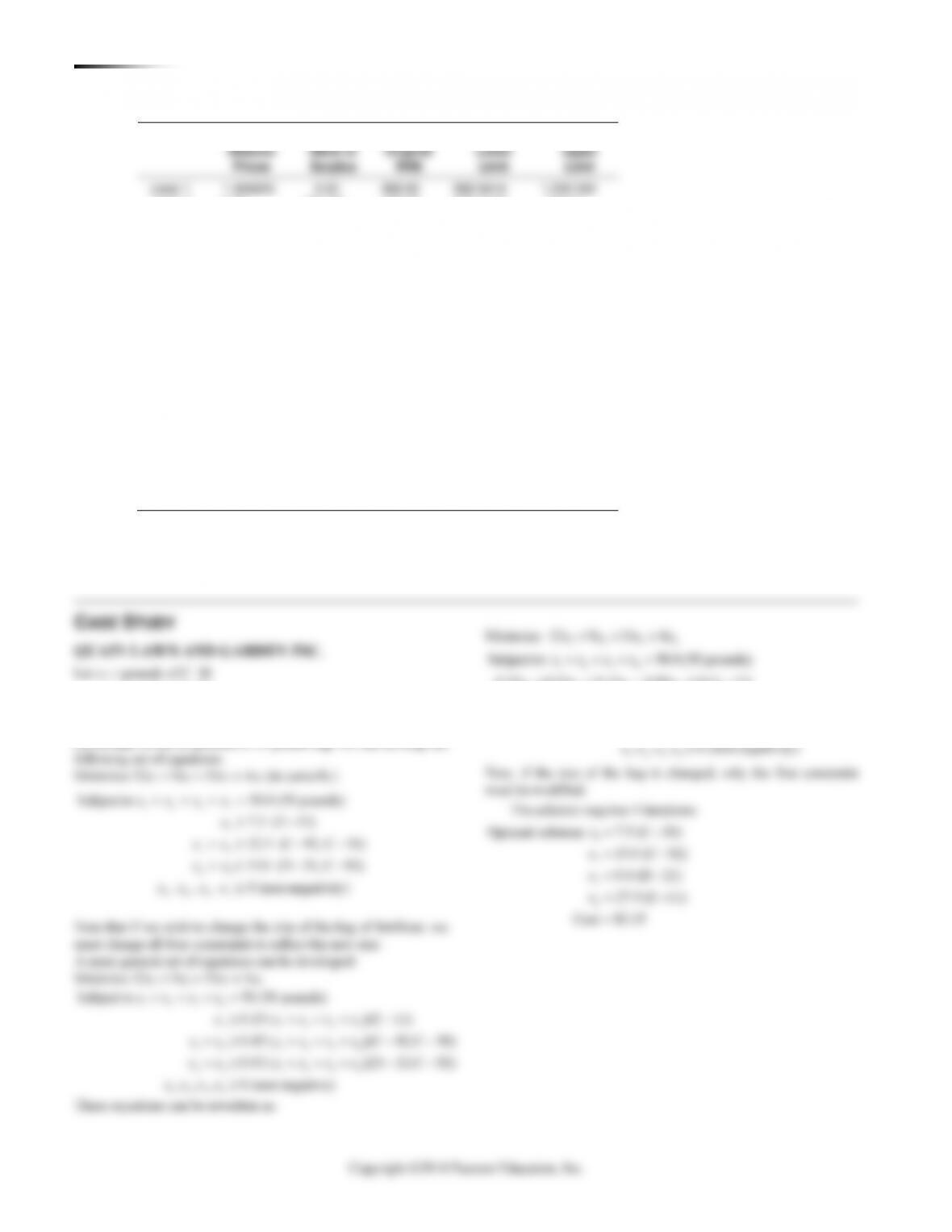
* The optimal solution is to make 262.5 benches and 25 tables per
period. Profit will be $2,862.50. Because benches and tables may
be matched (two benches per table), it may not be reasonable to
maximize profit in this manner. Also, this problem brings up the
proper interpretation of the statement “One should make 262.5
(a fractional quantity) benches per period.”
B.32
288 BUSINESS ANALYTICS MODULE B LIN E A R PR O G R A M M I N G
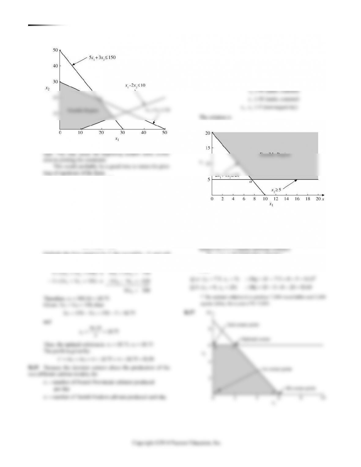
Note that this problem has one constraint with a negative
x1 − 2x2 10
found in this problem, and of the form:
3x1 − 2x2 0
The optimal point, a, lies at the intersection of the
constraints:
3x1 + 5x2 150
5x1 + 3x2 150
To solve these equations simultaneously, begin by writing
them in the form shown below:
3x1 + 5x2 = 150
5x1 + 3x2 = 150
Multiply the first equation by 5, the second by −3, and add
the two equations:
+ = → + =
1 2 1 2
5 (3 5 150) 15 25 750
x x x x
3x1 = 150 − 5x2 = 150 − 5 18.75
and
1
56.25 18.75
3
x==
Thus, the optimal solution is: x1 = 18.75, x2 = 18.75
x1 = number of French Provincial cabinets produced
per day
x2 = number of Danish Modern cabinets produced each day
The equations become:
Objective: 28x1 + 25x2 (maximize revenue)
12
12
12
1
2
12
Subject to 3 2 360 (hours, carpentry)
1.5 1 200 (hours, painting)
0.75 0.75 125 (hours, finishing)
60 (units, contract)
60 (units, contract)
, 0 (non-negativity)
xx
xx
xx
x
x
xx
+
+
+
The solution is:
x1 = 60, x2 = 90, Revenue = $3930/day
Define the following variables:
x1 = thousands of round tables produced per month
x2 = thousands of square tables produced per month
The appropriate equations then become:
Objective: 10x1 + 8x2 (minimize handling and storage costs)
2x1 + 1x2 20 (total labor capacity)
x1, x2 0 (non-negativity)
Cost:
*
@ : ( 7.5, 5) Obj 10 7.5 8 5 $115
a x x
= = = + =
B.34
B.36
B.37
290 BUSINESS ANALYTICS MODULE B LIN E A R PR O G R A M M I N G
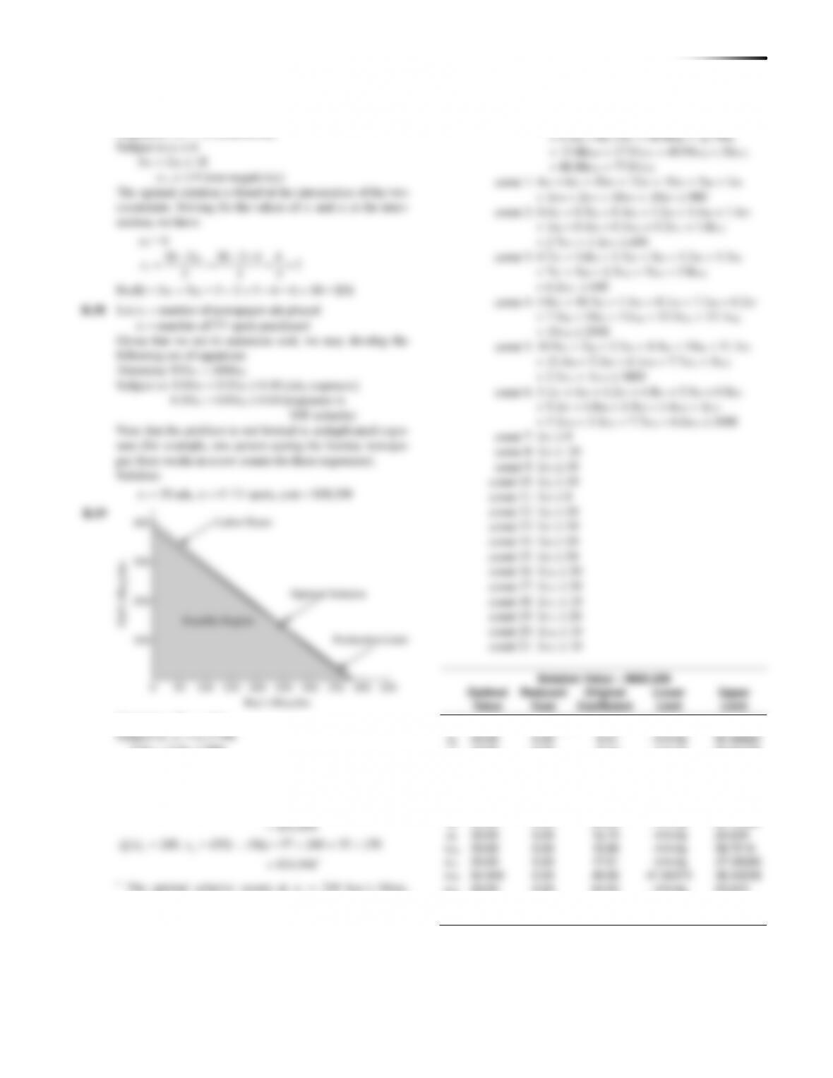
Solution Value = 9683.229
Shadow
Slack or
Original
Lower
Upper
Prices
Surplus
RHS
Limit
Limit
const 1
2.711812
0.00
980.00
861.5504
1,024.236
const 2
0.00
113.866
400.00
286.1337
Infinity
const 3
10.6486
0.00
600.00
587.7851
608.5712
const 4
2.182708
0.00
2,500.00
1,889.72
2,534.683
const 5
0.00
258.885
1,800.00
1,541.115
Infinity
const 6
0.00
8.52954
1,000.00
991.4705
Infinity
const 7
0.00
0.00
0.00
−Infinity
0.00
const 8
−46.1866
0.00
20.00
17.91737
41.84552
const 9
−26.4548
0.00
10.00
5.041353
19.9601
const 10
−2.53532
0.00
10.00
0.00
16.993
const 11
0.00
11.5072
0.00
−Infinity
11.50722
const 12
−27.37
0.00
20.00
16.50255
37.096
const 13
−34.041
10.00
10.00
3.532913
12.01538
const 14
−32.6758
0.00
20.00
17.09391
23.00434
const 15
−11.75
0.00
50.00
39.20661
116.4478
const 16
−10.8416
0.00
20.00
14.30611
79.923
const 17
−9.37385
0.00
20.00
15.88757
68.822
const 18
0.00
44.95
10.00
−Infinity
54.94591
const 19
−29.243
0.00
20.00
15.45261
22.44298
const 20
0.00
2.20215
10.00
−Infinity
12.20215
const 21
−48.87
0.00
10.00
8.355577
12.84913
The optimal solution provides a profit of $9683. Note that
only product A158 is not produced.
(b) The shadow prices are given in the table above.
(c) There is no value to adding more workers because those

BUSINESS ANALYTICS MODULE B LI N EA R PR O G R A M M I N G 291
Solution Value = 8865.5
Shadow
Slack or
Original
Lower
Upper
Prices
Surplus
RHS
Limit
Limit
const 1
2.74856
0.00
980.00
913.6641
993.1374
const 2
0.00
113.879
400.00
286.1211
Infinity
const 3
9.197201
0.00
600.00
587.7851
601.577
const 4
2.343288
0.00
2,500.00
2,342.00
2,512.443
const 5
0.00
266.934
1,800.00
1,533.066
Infinity
const 6
0.00
2.36523
1,000.00
997.6348
Infinity
const 7
0.00
0.00
0.00
−Infinity
0.00
const 8
−45.3751
0.00
20.00
19.45971
41.84552
const 9
−24.6748
0.00
10.00
8.988791
19.9601
const 10
0.00
6.993
10.00
−Infinity
16.993
const 11
0.00
7.05643
0.00
−Infinity
7.056433
const 12
−26.3331
0.00
20.00
19.15507
37.096
const 13
−25.2444
0.00
10.00
9.459686
12.01538
const 14
−26.7748
0.00
20.00
19.5257
23.00434
const 15
−13.3914
0.00
50.00
39.20661
62.76064
const 16
−12.6447
0.00
20.00
17.28464
31.80706
const 17
−11.3811
0.00
20.00
18.28127
32.64
const 18
0.00
47.70
10.00
−Infinity
57.69793
const 19
−21.986
0.00
20.00
19.46232
22.44298
const 20
71.9494
0.00
10.00
9.155032
12.20215
const 21
−42.6476
0.00
10.00
9.67822
12.84913
Note that the profit declines to $8,865 with the reduction in
contribution to $8.88.
x4 0, x5 0. The following results:
Solution Value = 9380.23
Optimal
Reduced
Original
Lower
Upper
Value
Cost
Coefficient
Limit
Limit
x1
0.00
7.90441
18.79
−Infinity
26.69441
x2
0.00
16.81
6.31
−Infinity
23.1219
x3
0.00
10.9491
8.19
−Infinity
19.1391
x4
0.00
2.75734
45.88
−Infinity
48.63734
x5
28.72255
0.00
63.00
61.75618
63.859
x6
20.00
0.00
4.10
−Infinity
12.95034
x7
10.00
0.00
81.15
−Infinity
86.86531
x8
37.51722
0.00
50.06
49.69948
71.07961
x9
50.00
0.00
12.79
−Infinity
23.18852
x10
20.00
0.00
15.88
−Infinity
20.73238
x11
33.94098
0.00
17.91
17.22904
18.570
x12
37.485
0.00
49.99
48.67592
51.016
x13
20.00
0.00
24.00
−Infinity
24.49456
x14
10.00
0.00
8.88
−Infinity
70.86956
x15
10.27741
0.00
77.01
75.18908
77.47366
292 BUSINESS ANALYTICS MODULE B LIN E A R PR O G R A M M I N G
Solution Value = 9380.234
Shadow
Slack or
Original
Lower
Upper
Prices
Surplus
RHS
Limit
Limit
const 1
1.494825
0.00
980.00
969.9414
1,202.002
const 2
0.00
120.755
400.00
279.2448
Infinity
const 3
0.7247843
0.00
600.00
598.0171
811.0541
const 4
0.8810187
0.00
2,500.00
2492.973
2,917.931
const 5
0.0234673
0.00
1,800.00
1530.888
1,805.481
const 6
6.716568
0.00
1,000.00
918.2866
1,002.674
const 7
0.00
0.00
0.00
−Infinity
0.00
const 8
0.00
0.00
0.00
−Infinity
0.00
const 9
0.00
0.00
0.00
−Infinity
0.00
const 10
0.00
0.00
0.00
−Infinity
0.00
const 11
0.00
28.7226
0.00
−Infinity
28.72255
const 12
−8.85034
0.00
20.00
17.19764
40.10845
const 13
−5.71531
0.00
10.00
0.00
25.09986
const 14
0.00
17.5172
20.00
−Infinity
37.51723
const 15
−10.3985
0.00
50.00
42.69018
75.98374
const 16
−4.85238
0.00
20.00
0.00
38.00887
const 17
0.00
13.94
20.00
−Infinity
33.94098
const 18
0.00
27.4846
10.00
−Infinity
37.485
const 19
−0.494562
0.00
20.00
1.392963
21.02138
const 20
−61.9896
0.00
10.00
0.7036638
10.96196
const 21
0.00
0.2774
10.00
−Infinity
10.27741
Profit increases to $9,380, and none of the products
beginning with A–D remain.
Previously, only A158 was not produced.
x2 = pounds of C–92
x3 = pounds of D–21
x4 = pounds of E–11
Given that we are to produce a 50-pound bag, we can develop the
following set of equations:
1 2 3 4
4
Subject to 50.0 (50 pounds)
7.5 (E 11)
x x x x
x
+ + + =
−
1 2 3 4
4 1 2 3 4
1 2 1 2 3 4
2 3 1 2 3 4
1 2 3 4
Subject to 50 (50 pounds)
0.15 ( )(E 11)
0.45 ( )(C 92,C 30)
0.03 ( )(D 21,C 92)
, , , 0 (non-negative)
x x x x
x x x x x
x x x x x x
x x x x x x
x x x x
+ + + =
+ + + −
+ + + + − −
+ + + + − −
These equations can be rewritten as:
1 2 3 4
1 2 3 4
1 2 3 4
1 2 3 4
0.15 0.15 0.15 0.85 0 (E 11)
0.55 0.55 0.45 0.45 0 (C 92,C 30)
0.30 0.70 0.70 0.30 0 (D 21,C 92)
, , , 0 (non-negativity)
x x x x
x x x x
x x x x
x x x x
+ + − −
− − + + − −
− − + − −
must be modified.
The solution requires 4 iterations:
=−
1
Optimal solution: 7.5 (C 30)
x
294 BUSINESS ANALYTICS MODULE B LI N EA R PR O G R A M M I N G
hour of the day are assumed to be deterministic. In a real situation,
wide fluctuations will be experienced in a stochastic manner.
The optimal solution results in a considerable amount of idle
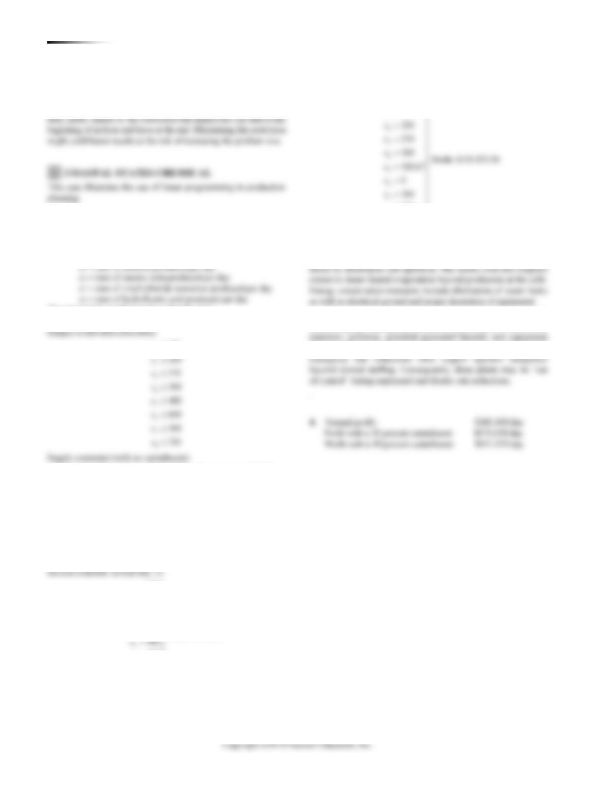
1. To develop the model:
Let: x1 = tons of phosphoric acid produced per day
x2 = tons of urea produced per day
x3 = tons of ammonium phosphate produced per day
x4 = tons of ammonium nitrate produced per day
The appropriate model equations then become:
Maximize 60x1 + 80x2 + 90x3 + 100x4 + 50x5 + 50x6 + 65x7 + 70x8
1
6
7
8
320
600
300
320
x
x
x
x
Supply constraint (with no curtailment):
5.5x1 + 7x2 + 8x3 + 10x4 + 15x5 + 16x6 + 12x7 + 11x8 36,000
(a) Supply constraint (20 percent gas curtailment):
5.5x1 + 7x2 + 8x3 + 10x4 + 15x5 + 16x6 + 12x7 + 11x8 28,800
(Note: 36,000 cu. ft. 103 0.80 = 28,800 cu. ft. 103)
(b) Supply constraints (40 percent gas curtailment):
5.5x1 + 7x2 + 8x3 + 10x4 + 15x5 + 16x6 + 12x7 + 11x8 21,600
(Note: 36,000 cu. ft. 103 0.60 = 21,600 cu. ft. 103)
With a 20 percent natural gas curtailment, the optimal pro-
1
2
3
4
5
6
7
8
320
200
270
300 Profit: $174,650
480
385
300
320
x
x
x
x
x
x
x
x
=
=
=
=
=
=
=
=
With a 40 percent natural gas curtailment, the optimal pro-
duction schedule, in tons/day, is:
1
8
320
320
x
x
=
=
2. Obviously, those products that have high energy consumption
factors must undergo extensive scrutiny to conserve energy. These
products include chlorine (15.0) and caustic soda (16.0). Energy
consumption is high for these chemicals because they are pro-
3. These products are all produced by large-volume, capital-
intensive plants. Emergency shutdowns often result in loss of raw
materials, pollution, potential personnel hazards, and equipment
damage. These plants are staffed for normal operations, and
4. Normal profit: $185,400/day
Profit with a 20 percent curtailment: $174,650/day
Profit with a 40 percent curtailment: $151,933/day
BUSINESS ANALYTICS MODULE B LI N EA R PR O G R A M M I N G 287
12
*
12
12
@ : ( 0, 100) Obj 9 0 20 100 $2,000.00
@ : ( 262.5, 25) Obj 9 262.5 20 25 $2,862.50
@ : ( 300, 0) Obj 9 300 20 0 $2,700.00
a x x
b x x
c x x
= = = + =
= = = + =
= = = + =
ADDITIONAL HOMEWORK PROBLEMS
Here are the answers to additional homework problems
B.31–B.40 that appear on our Web sites, www.myomlab.com and
at www.pearsonhighered.com/heizer.
B.31 Let x = number of standard model to produce
y = number of deluxe model to produce
Maximize 40x + 60y
Subject to 30 30 450
10 15 180
6
xy
xy
x
+
+
Feasible corner points (x,y): (6,0), (15,0), (6,8), (9,6). Max-
imum profit is $720 by producing either 6 standard and
8 deluxe or 9 standard and 6 deluxe.
B.33
x2 = number of tables produced
Maximize 9x1 + 20x2
Subject to 4x1 + 6x2 1,200 (hours)
10x1 + 35x2 3,500 (board-feet)
x1, x2 0 (non-negativity)
Profit:
Adjustable cells
Sensitivity Report (Relevant Section)
Cell
Name
Final
Value
Reduced
Cost
Objective
Coefficient
Allowable
Increase
Allowable
Decrease
$B$14
serving AS
0
0.1726
0.3
1E + 30
0.1726
$C$14
serving CC
1.333
0
0.4
0.2589
0.2256
$D$14
serving FC
0.457
0
0.9
0.1051
0.1006
$E$14
serving FF
0
0.1527
0.2
1E + 30
0.1529
$F$14
serving M
1.130
0
0.5
0.0629
0.7078
$G$14
serving TB
0
0.1693
1.5
1E + 30
0.1694
$H$14
serving GS
0
0.6661
0.9
1E + 30
0.6882
Constraints
Cell
Name
Final
Value
Shadow
Price
Constraint
R.H. Side
Allowable
Increase
Allowable
Decrease
$I$17
Cals min LI
800
0
500
300
1E + 30
$I$18
Cals max L
800
– 0.00023
800
200
251.6129
$I$19
Protein min
200
0.008983
200
155
40
$I$20
Carb min L
311.43
0
200
111.4285
1E + 30
$I$21
Fat max LI
288.57
0
400
1E + 30
111.4286
$I$22
Fruit + Veg I
200
0.0015
200
485.7143
200
* The optimal solution is to make 262.5 benches and 25 tables per
period. Profit will be $2,862.50. Because benches and tables may
be matched (two benches per table), it may not be reasonable to
maximize profit in this manner. Also, this problem brings up the
proper interpretation of the statement “One should make 262.5
(a fractional quantity) benches per period.”
B.32
288 BUSINESS ANALYTICS MODULE B LIN E A R PR O G R A M M I N G
Note that this problem has one constraint with a negative
x1 − 2x2 10
found in this problem, and of the form:
3x1 − 2x2 0
The optimal point, a, lies at the intersection of the
constraints:
3x1 + 5x2 150
5x1 + 3x2 150
To solve these equations simultaneously, begin by writing
them in the form shown below:
3x1 + 5x2 = 150
5x1 + 3x2 = 150
Multiply the first equation by 5, the second by −3, and add
the two equations:
+ = → + =
1 2 1 2
5 (3 5 150) 15 25 750
x x x x
3x1 = 150 − 5x2 = 150 − 5 18.75
and
1
56.25 18.75
3
x==
Thus, the optimal solution is: x1 = 18.75, x2 = 18.75
x1 = number of French Provincial cabinets produced
per day
x2 = number of Danish Modern cabinets produced each day
The equations become:
Objective: 28x1 + 25x2 (maximize revenue)
12
12
12
1
2
12
Subject to 3 2 360 (hours, carpentry)
1.5 1 200 (hours, painting)
0.75 0.75 125 (hours, finishing)
60 (units, contract)
60 (units, contract)
, 0 (non-negativity)
xx
xx
xx
x
x
xx
+
+
+
The solution is:
x1 = 60, x2 = 90, Revenue = $3930/day
Define the following variables:
x1 = thousands of round tables produced per month
x2 = thousands of square tables produced per month
The appropriate equations then become:
Objective: 10x1 + 8x2 (minimize handling and storage costs)
2x1 + 1x2 20 (total labor capacity)
x1, x2 0 (non-negativity)
Cost:
*
@ : ( 7.5, 5) Obj 10 7.5 8 5 $115
a x x
= = = + =
B.34
B.36
B.37
290 BUSINESS ANALYTICS MODULE B LIN E A R PR O G R A M M I N G
Solution Value = 9683.229
Shadow
Slack or
Original
Lower
Upper
Prices
Surplus
RHS
Limit
Limit
const 1
2.711812
0.00
980.00
861.5504
1,024.236
const 2
0.00
113.866
400.00
286.1337
Infinity
const 3
10.6486
0.00
600.00
587.7851
608.5712
const 4
2.182708
0.00
2,500.00
1,889.72
2,534.683
const 5
0.00
258.885
1,800.00
1,541.115
Infinity
const 6
0.00
8.52954
1,000.00
991.4705
Infinity
const 7
0.00
0.00
0.00
−Infinity
0.00
const 8
−46.1866
0.00
20.00
17.91737
41.84552
const 9
−26.4548
0.00
10.00
5.041353
19.9601
const 10
−2.53532
0.00
10.00
0.00
16.993
const 11
0.00
11.5072
0.00
−Infinity
11.50722
const 12
−27.37
0.00
20.00
16.50255
37.096
const 13
−34.041
10.00
10.00
3.532913
12.01538
const 14
−32.6758
0.00
20.00
17.09391
23.00434
const 15
−11.75
0.00
50.00
39.20661
116.4478
const 16
−10.8416
0.00
20.00
14.30611
79.923
const 17
−9.37385
0.00
20.00
15.88757
68.822
const 18
0.00
44.95
10.00
−Infinity
54.94591
const 19
−29.243
0.00
20.00
15.45261
22.44298
const 20
0.00
2.20215
10.00
−Infinity
12.20215
const 21
−48.87
0.00
10.00
8.355577
12.84913
The optimal solution provides a profit of $9683. Note that
only product A158 is not produced.
(b) The shadow prices are given in the table above.
(c) There is no value to adding more workers because those
BUSINESS ANALYTICS MODULE B LI N EA R PR O G R A M M I N G 291
Solution Value = 8865.5
Shadow
Slack or
Original
Lower
Upper
Prices
Surplus
RHS
Limit
Limit
const 1
2.74856
0.00
980.00
913.6641
993.1374
const 2
0.00
113.879
400.00
286.1211
Infinity
const 3
9.197201
0.00
600.00
587.7851
601.577
const 4
2.343288
0.00
2,500.00
2,342.00
2,512.443
const 5
0.00
266.934
1,800.00
1,533.066
Infinity
const 6
0.00
2.36523
1,000.00
997.6348
Infinity
const 7
0.00
0.00
0.00
−Infinity
0.00
const 8
−45.3751
0.00
20.00
19.45971
41.84552
const 9
−24.6748
0.00
10.00
8.988791
19.9601
const 10
0.00
6.993
10.00
−Infinity
16.993
const 11
0.00
7.05643
0.00
−Infinity
7.056433
const 12
−26.3331
0.00
20.00
19.15507
37.096
const 13
−25.2444
0.00
10.00
9.459686
12.01538
const 14
−26.7748
0.00
20.00
19.5257
23.00434
const 15
−13.3914
0.00
50.00
39.20661
62.76064
const 16
−12.6447
0.00
20.00
17.28464
31.80706
const 17
−11.3811
0.00
20.00
18.28127
32.64
const 18
0.00
47.70
10.00
−Infinity
57.69793
const 19
−21.986
0.00
20.00
19.46232
22.44298
const 20
71.9494
0.00
10.00
9.155032
12.20215
const 21
−42.6476
0.00
10.00
9.67822
12.84913
Note that the profit declines to $8,865 with the reduction in
contribution to $8.88.
x4 0, x5 0. The following results:
Solution Value = 9380.23
Optimal
Reduced
Original
Lower
Upper
Value
Cost
Coefficient
Limit
Limit
x1
0.00
7.90441
18.79
−Infinity
26.69441
x2
0.00
16.81
6.31
−Infinity
23.1219
x3
0.00
10.9491
8.19
−Infinity
19.1391
x4
0.00
2.75734
45.88
−Infinity
48.63734
x5
28.72255
0.00
63.00
61.75618
63.859
x6
20.00
0.00
4.10
−Infinity
12.95034
x7
10.00
0.00
81.15
−Infinity
86.86531
x8
37.51722
0.00
50.06
49.69948
71.07961
x9
50.00
0.00
12.79
−Infinity
23.18852
x10
20.00
0.00
15.88
−Infinity
20.73238
x11
33.94098
0.00
17.91
17.22904
18.570
x12
37.485
0.00
49.99
48.67592
51.016
x13
20.00
0.00
24.00
−Infinity
24.49456
x14
10.00
0.00
8.88
−Infinity
70.86956
x15
10.27741
0.00
77.01
75.18908
77.47366
292 BUSINESS ANALYTICS MODULE B LIN E A R PR O G R A M M I N G
Solution Value = 9380.234
Shadow
Slack or
Original
Lower
Upper
Prices
Surplus
RHS
Limit
Limit
const 1
1.494825
0.00
980.00
969.9414
1,202.002
const 2
0.00
120.755
400.00
279.2448
Infinity
const 3
0.7247843
0.00
600.00
598.0171
811.0541
const 4
0.8810187
0.00
2,500.00
2492.973
2,917.931
const 5
0.0234673
0.00
1,800.00
1530.888
1,805.481
const 6
6.716568
0.00
1,000.00
918.2866
1,002.674
const 7
0.00
0.00
0.00
−Infinity
0.00
const 8
0.00
0.00
0.00
−Infinity
0.00
const 9
0.00
0.00
0.00
−Infinity
0.00
const 10
0.00
0.00
0.00
−Infinity
0.00
const 11
0.00
28.7226
0.00
−Infinity
28.72255
const 12
−8.85034
0.00
20.00
17.19764
40.10845
const 13
−5.71531
0.00
10.00
0.00
25.09986
const 14
0.00
17.5172
20.00
−Infinity
37.51723
const 15
−10.3985
0.00
50.00
42.69018
75.98374
const 16
−4.85238
0.00
20.00
0.00
38.00887
const 17
0.00
13.94
20.00
−Infinity
33.94098
const 18
0.00
27.4846
10.00
−Infinity
37.485
const 19
−0.494562
0.00
20.00
1.392963
21.02138
const 20
−61.9896
0.00
10.00
0.7036638
10.96196
const 21
0.00
0.2774
10.00
−Infinity
10.27741
Profit increases to $9,380, and none of the products
beginning with A–D remain.
Previously, only A158 was not produced.
x2 = pounds of C–92
x3 = pounds of D–21
x4 = pounds of E–11
Given that we are to produce a 50-pound bag, we can develop the
following set of equations:
1 2 3 4
4
Subject to 50.0 (50 pounds)
7.5 (E 11)
x x x x
x
+ + + =
−
1 2 3 4
4 1 2 3 4
1 2 1 2 3 4
2 3 1 2 3 4
1 2 3 4
Subject to 50 (50 pounds)
0.15 ( )(E 11)
0.45 ( )(C 92,C 30)
0.03 ( )(D 21,C 92)
, , , 0 (non-negative)
x x x x
x x x x x
x x x x x x
x x x x x x
x x x x
+ + + =
+ + + −
+ + + + − −
+ + + + − −
These equations can be rewritten as:
1 2 3 4
1 2 3 4
1 2 3 4
1 2 3 4
0.15 0.15 0.15 0.85 0 (E 11)
0.55 0.55 0.45 0.45 0 (C 92,C 30)
0.30 0.70 0.70 0.30 0 (D 21,C 92)
, , , 0 (non-negativity)
x x x x
x x x x
x x x x
x x x x
+ + − −
− − + + − −
− − + − −
must be modified.
The solution requires 4 iterations:
=−
1
Optimal solution: 7.5 (C 30)
x
294 BUSINESS ANALYTICS MODULE B LI N EA R PR O G R A M M I N G
hour of the day are assumed to be deterministic. In a real situation,
wide fluctuations will be experienced in a stochastic manner.
The optimal solution results in a considerable amount of idle
1. To develop the model:
Let: x1 = tons of phosphoric acid produced per day
x2 = tons of urea produced per day
x3 = tons of ammonium phosphate produced per day
x4 = tons of ammonium nitrate produced per day
The appropriate model equations then become:
Maximize 60x1 + 80x2 + 90x3 + 100x4 + 50x5 + 50x6 + 65x7 + 70x8
1
6
7
8
320
600
300
320
x
x
x
x
Supply constraint (with no curtailment):
5.5x1 + 7x2 + 8x3 + 10x4 + 15x5 + 16x6 + 12x7 + 11x8 36,000
(a) Supply constraint (20 percent gas curtailment):
5.5x1 + 7x2 + 8x3 + 10x4 + 15x5 + 16x6 + 12x7 + 11x8 28,800
(Note: 36,000 cu. ft. 103 0.80 = 28,800 cu. ft. 103)
(b) Supply constraints (40 percent gas curtailment):
5.5x1 + 7x2 + 8x3 + 10x4 + 15x5 + 16x6 + 12x7 + 11x8 21,600
(Note: 36,000 cu. ft. 103 0.60 = 21,600 cu. ft. 103)
With a 20 percent natural gas curtailment, the optimal pro-
1
2
3
4
5
6
7
8
320
200
270
300 Profit: $174,650
480
385
300
320
x
x
x
x
x
x
x
x
=
=
=
=
=
=
=
=
With a 40 percent natural gas curtailment, the optimal pro-
duction schedule, in tons/day, is:
1
8
320
320
x
x
=
=
2. Obviously, those products that have high energy consumption
factors must undergo extensive scrutiny to conserve energy. These
products include chlorine (15.0) and caustic soda (16.0). Energy
consumption is high for these chemicals because they are pro-
3. These products are all produced by large-volume, capital-
intensive plants. Emergency shutdowns often result in loss of raw
materials, pollution, potential personnel hazards, and equipment
damage. These plants are staffed for normal operations, and
4. Normal profit: $185,400/day
Profit with a 20 percent curtailment: $174,650/day
Profit with a 40 percent curtailment: $151,933/day


