CHAPTER 9
OPTIMIZATION IN DESIGN AND OPERATIONS
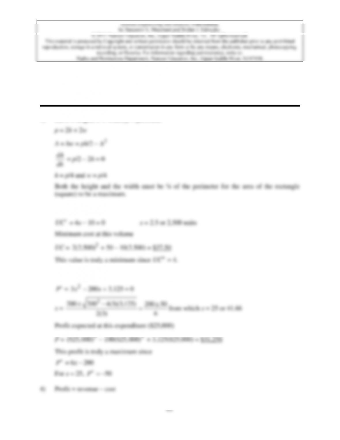
1) Let h = height; w = width; p = perimeter
2) Value of x for minimum unit cost
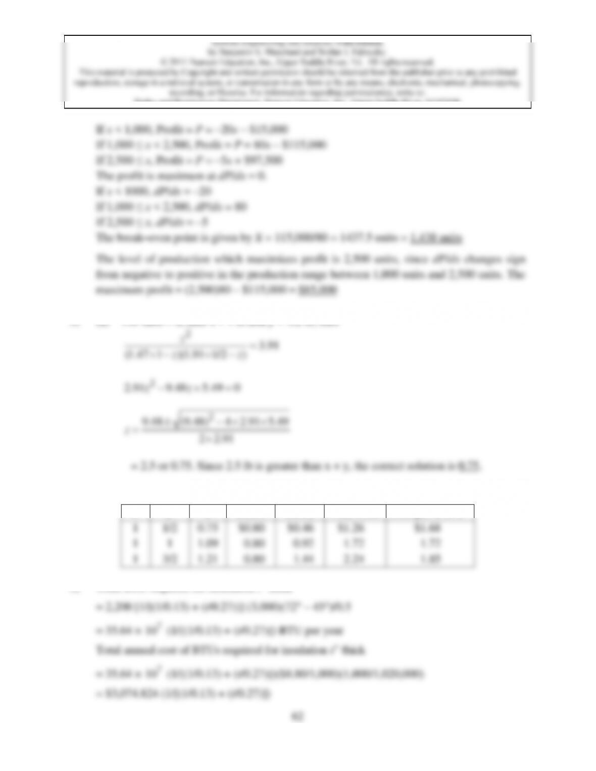
3) Advertising expenditure which maximizes profit is found from
2
Rights and Permissions Department, Pearson Education, Inc., Upper Saddle River, NJ 07458.
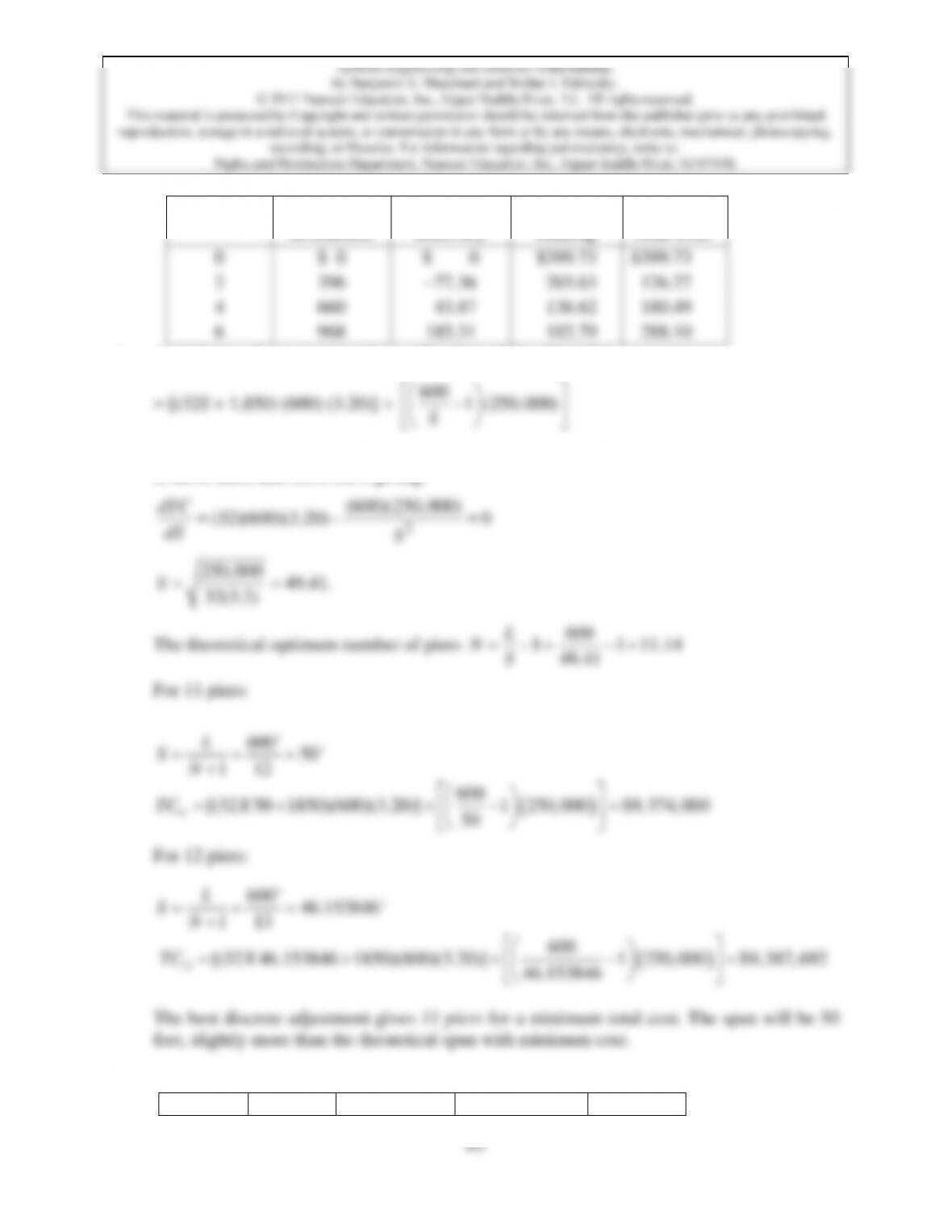
Thickness
Initial
Investment
Capital
Recovery
Cost of
Heating
Total Cost
0
$ 0
$ 0
$399.73
$399.73
2
396
–77.36
203.63
126.27
4
660
43.87
136.62
180.49
6
968
185.31
102.79
288.10
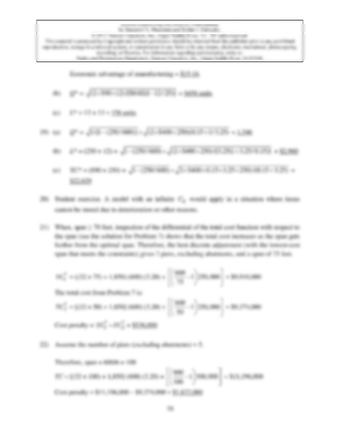
7) Total Cost = Superstructure Cost + Pier Cost, TC = SC + PC
600 1 (250, 000)
S
To find the optimum span between piers, differentiate the total cost function with respect to
S, set to zero, and solve for S giving:
(600)(250,000)
dTC
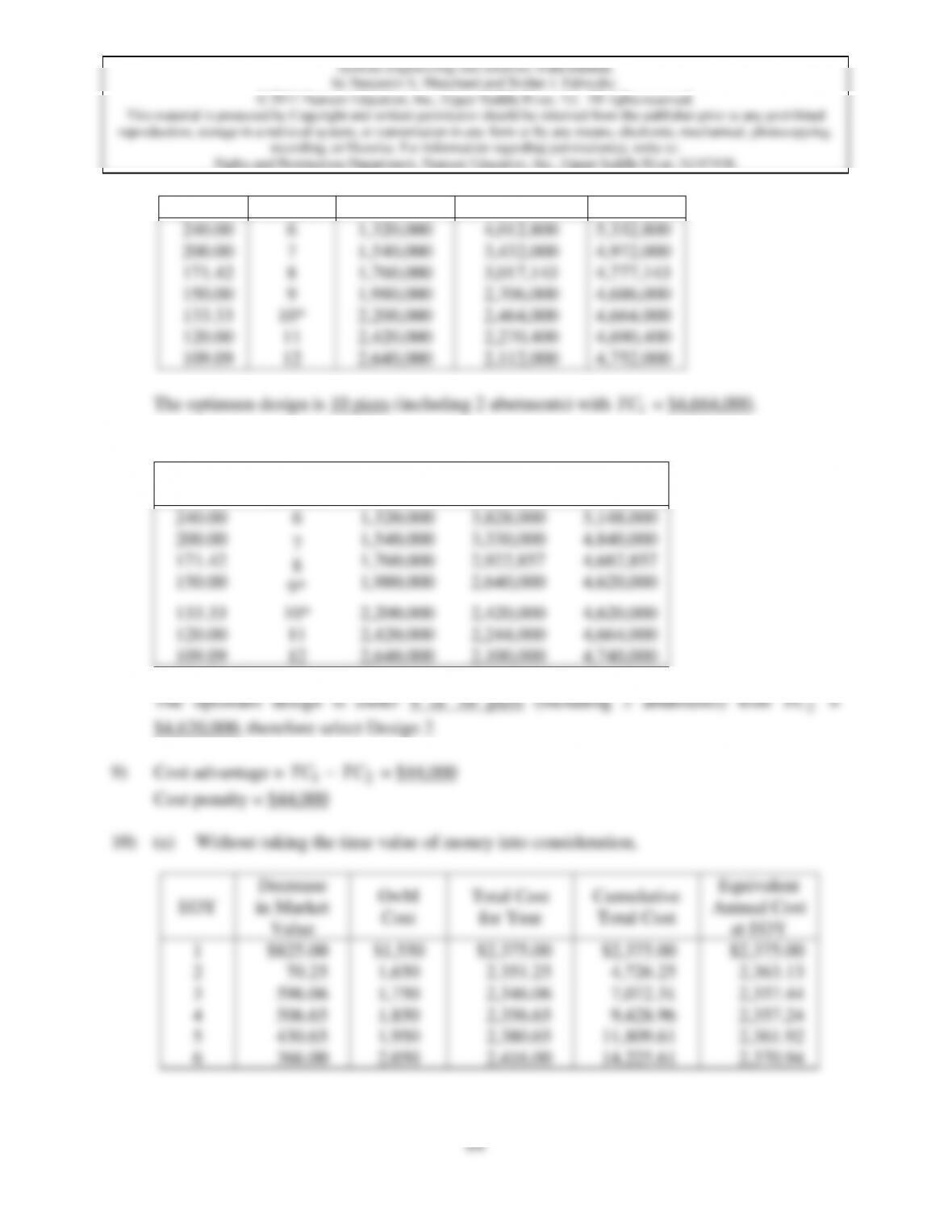
8) Tabular solution for Design 1:
Span
Number
Pier Cost
Superstructure
Total
1
TC
$1,550
$2,375.00
$2,375.00
2,351.25
4,726.25
2,363.13
2,346.06
7,072.31
2,357.44
2,356.65
9,428.96
2,357.24
2,380.65
11,809.61
2,361.92
2,416.00
14,225.61
2,370.94
in Feet
of Piers
($)
Cost ($)
Cost ($)
240.00
6
1,320,000
4,012,800
5,332,800
200.00
7
1,540,000
3,432,000
4,972,000
171.42
8
1,760,000
3,017,143
4,777,143
150.00
9
1,980,000
2,706,000
4,686,000
133.33
10*
2,200,000
2,464,000
4,664,000
120.00
11
2,420,000
2,270,400
4,690,400
109.09
12
2,640,000
2,112,000
4,752,000
The optimum design is 10 piers (including 2 abutments) with
1
TC
= $4,664,000.
Tabular solution for Design 2:
Span
(Feet)
Number
of Piers
Pier Cost
($)
Superstructure
Cost ($)
Total Cost
($)
240.00
6
1,320,000
3,828,000
5,148,000
200.00
171.42
150.00
7
8
9*
1,540,000
1,760,000
1,980,000
3,330,000
2,922,857
2,640,000
4,840,000
4,682,857
4,620,000
133.33
10*
2,200,000
2,420,000
4,620,000
120.00
11
2,420,000
2,244,000
4,664,000
109.09
12
2,640,000
2,100,000
4,740,000
65
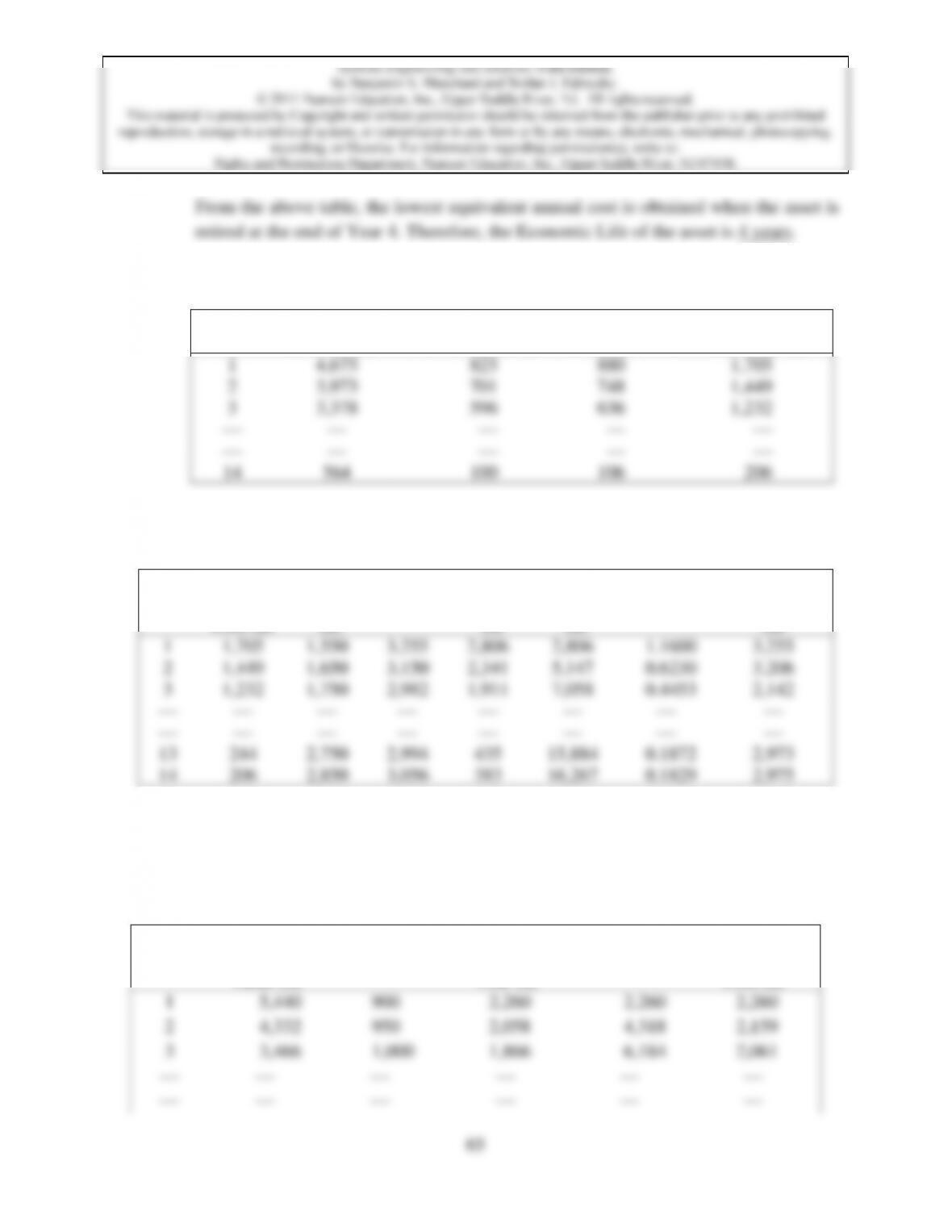
From the above table, the lowest equivalent annual cost is obtained when the asset is
retired at the end of Year 4. Therefore, the Economic Life of the asset is 4 years.
(b) Capital recovery cost calculations with an interest rate = 16%:
EOY
Market value
at EOY ($)
Decrease in
Market Value ($)
Interest on
Investment
Capital Recovery
Cost for Year ($)
1
4,675
825
880
1,705
2
3,973
701
748
1,449
3
3,378
596
636
1,232
—
—
—
—
—
—
—
—
—
—
14
564
100
106
206
Sample calculations for Economic Life of the asset:
EOY
Capital
Recovery
Cost ($)
O+M
Cost
($)
Total
Cost ($)
PE
Cost
($)
Sum of
PE Cost
($)
(A/P
16%, N)
Equivalent
Annual Cost
($)
1
1,705
1,550
3,255
2,806
2,806
1.1600
3,255
2
1,449
1,650
3,150
2,341
5,147
0.6230
3,206
3
1,232
1,750
2,982
1,911
7,058
0.4453
2,142
—
—
—
—
—
—
—
—
—
—
—
—
—
—
—
—
13
244
2,750
2,994
435
15,884
0.1872
2,973
14
206
2,850
3,056
383
16,267
0.1829
2,975
From the calculations above, the lowest Equivalent Annual Cost occurs when the asset is
retired at the end of year 12. This is the Economic Life.
11) (a) Without taking the time value of money into consideration, the calculation is:
EOY
Decrease in
Market
Value ($)
O+M Cost
($)
Total Cost
for the
Year ($)
Cum. Total
Cost ($)
Equivalent
Annual
Cost ($)
1
5,440
900
2,260
2,260
2,260
2
4,332
950
2,058
4,318
2,159
3
3,466
1,000
1,866
6,184
2,061
—
—
—
—
—
—
—
—
—
—
—
—
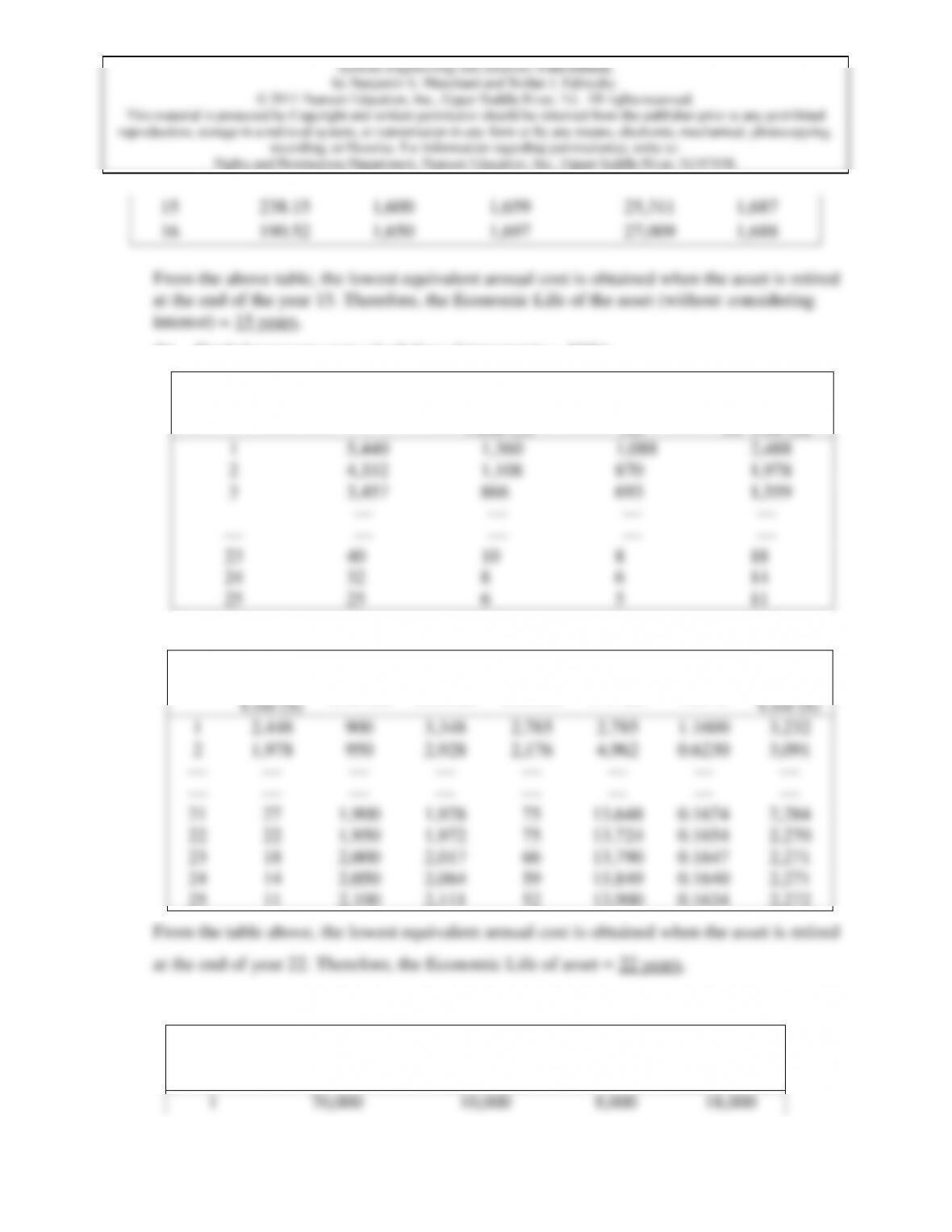
66
15
238.15
1,600
1,659
25,311
1,687
16
190.52
1,650
1,697
27,009
1,688
From the above table, the lowest equivalent annual cost is obtained when the asset is retired
at the end of the year 15. Therefore, the Economic Life of the asset (without considering
interest) = 15 years.
(b) Capital recovery cost calculations (interest rate = 16%):
EOY
Market Value
at EOY ($)
Decrease
in Market
Value ($)
Interest on
Investment
($)
Capital Re-
covery Cost
for Year ($)
1
5,440
1,360
1,088
2,488
2
4,332
1,108
870
1,978
3
3,457
866
693
1,559
—
—
—
—
—
—
—
—
—
23
40
10
8
18
24
32
8
6
14
25
25
6
5
11
Calculations for Economic Life of asset:
EOY
Capital
Recover
Cost ($)
O+M
Cost ($)
Total
Cost ($)
PE
Cost ($)
Cum.
PW ($)
(A/P,
16, N)
Equiv.
Annual
Cost ($)
1
2,448
900
3,348
2,785
2,785
1.1600
3,232
2
1,978
950
2,928
2,176
4,962
0.6230
3,091
—
—
—
—
—
—
—
—
—
—
—
—
—
—
—
—
21
27
1,900
1,928
75
13,648
0.1674
2,284
22
22
1,950
1,972
75
13,724
0.1654
2,270
23
18
2,000
2,017
66
13,790
0.1647
2,271
24
14
2,050
2,064
59
13,849
0.1640
2,271
25
11
2,100
2,111
52
13,900
0.1634
2,272
From the table above, the lowest equivalent annual cost is obtained when the asset is retired
at the end of year 22. Therefore, the Economic Life of asset = 22 years.
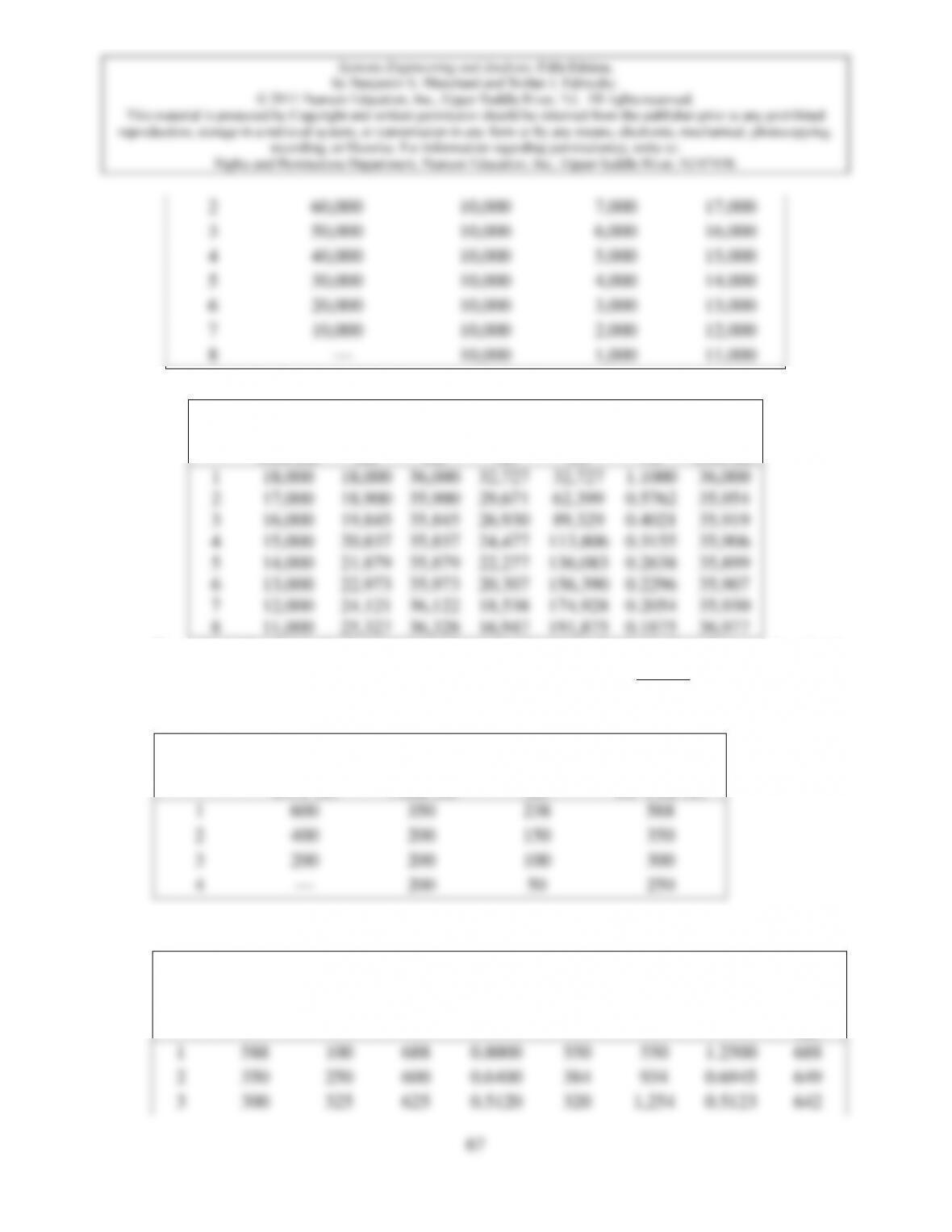
12) Capital recovery cost calculations (interest rate = 10%):
EOY
Market Value
at EOY ($)
Decrease
In Market
Value ($)
Interest on
Investment ($)
Capital Re-
covery Cost
for Year ($)
1
70,000
10,000
8,000
18,000
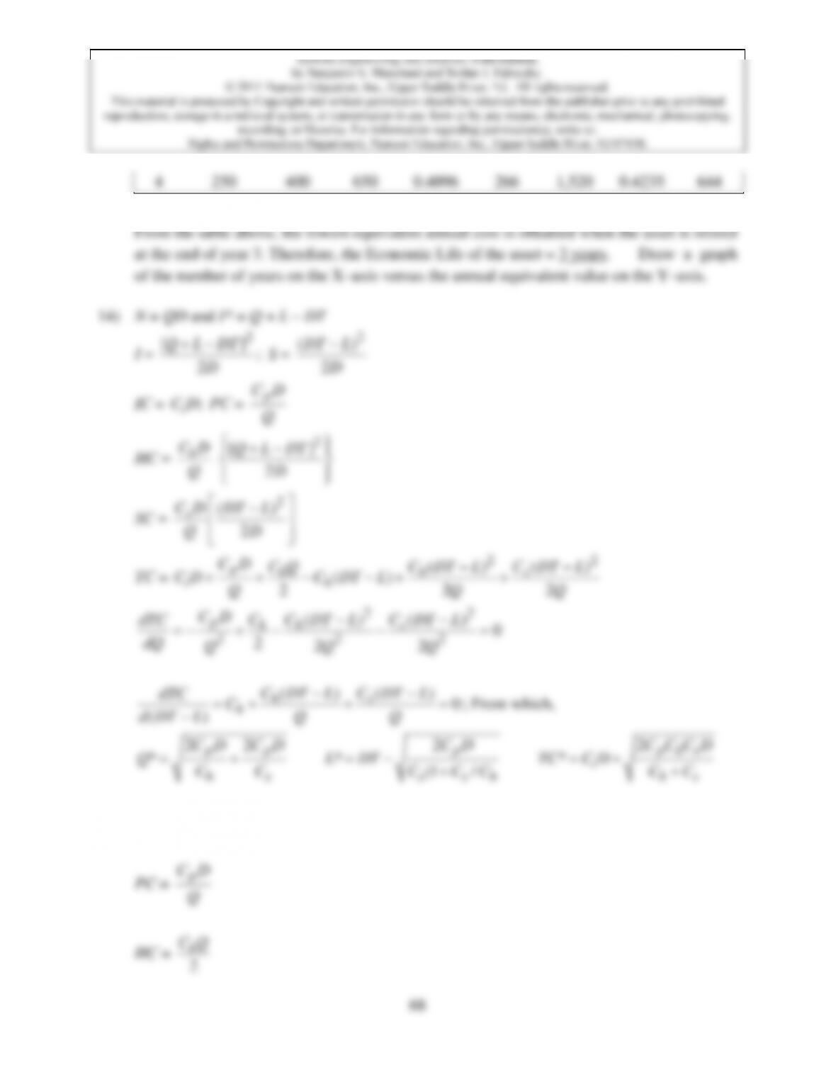
TC =
2
ph
i
CD CQ
CD Q
++
0
22
ph
CD C
dTC
dQ = + =
2
*p
h
CD
QC
=
*L DT=
TC* =
2/
2
2/
h p h
p
i
ph
C C D C
CD
CD C D C
++
=
2
i p h
C D C C D+
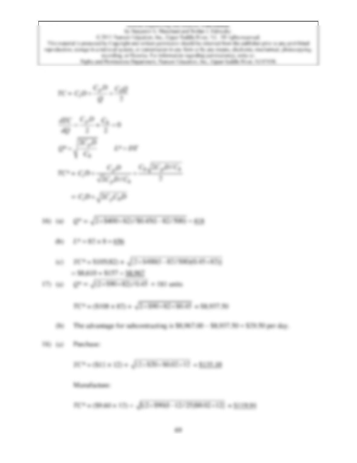
16) (a) Q* =
2 $400 82) / $0.45(1 82 / 500) 418 − =
(b) L* = 82 × 8 = 656
(c) TC* = $105(82) +
[2 $400(1 82/ 500)(0.45 82)] −
= $8,610 + $157 = $8,967
17) (a) Q* =
(2 $90 82) / 0.45
= 181 units
TC* = ($108 × 82) +
2 $90 82 $0.45
= $8,937.50
(b) The advantage for subcontracting is $8,967.00 – $8,937.50 = $29.50 per day.
18) (a) Purchase:
TC* = ($11 × 12) +
(2 $20 $0.02 12
= $135.10
Manufacture:
TC* = ($9.60 × 12) +
[(2 $90(1 12 / 25)$0.02 12] −
= $119.94
Rights and Permissions Department, Pearson Education, Inc., Upper Saddle River, NJ 07458.
70
0
15
30
45
y
2.4x + 3.2y = 140
0.0x + 2.6y = 80
4.1x + 0.0y = 120
Iso–value line
15 30 45 60
x
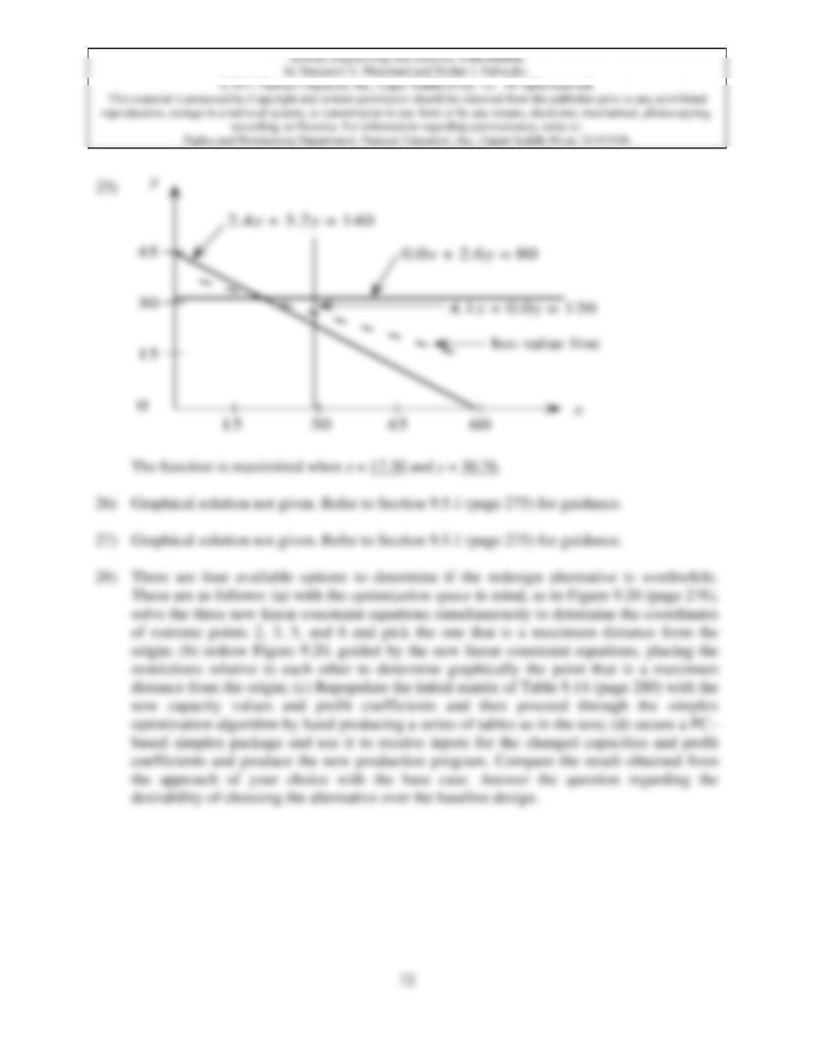
The function is maximized when x = 17.30 and y = 30.76.
26) Graphical solution not given. Refer to Section 9.5.1 (page 275) for guidance.
27) Graphical solution not given. Refer to Section 9.5.1 (page 275) for guidance.
28) There are four available options to determine if the redesign alternative is worthwhile.
These are as follows: (a) with the optimization space in mind, as in Figure 9.20 (page 278),
solve the three new linear constraint equations simultaneously to determine the coordinates
of extreme points 2, 3, 5, and 6 and pick the one that is a maximum distance from the
origin; (b) redraw Figure 9.20, guided by the new linear constraint equations, placing the
restrictions relative to each other to determine graphically the point that is a maximum
distance from the origin; (c) Repopulate the initial matrix of Table 9.14 (page 280) with the
new capacity values and profit coefficients and then proceed through the simplex
optimization algorithm by hand producing a series of tables as in the text; (d) secure a PC–
based simplex package and use it to receive inputs for the changed capacities and profit
coefficients and produce the new production program. Compare the result obtained from
the approach of your choice with the base case. Answer the question regarding the
desirability of choosing the alternative over the baseline design.
25)