CHAPTER 17
DESIGN FOR AFFORDABILITY
(LIFE – CYCLE COSTING)
1) Life–cycle cost (LCC) includes the total cost of a system over its entire life cycle. LCC
includes all of the costs associated with the activities identified in Figure 17.1 (page 568),
including the visible and the not so visible as in Figure 17.2 (page 569). When performing a
LCC analysis, all “future” research and development costs, production and/or construction
costs, operation and maintenance and support costs, retirement and material
recycling/disposal costs are to be identified and considered in the evaluation process. “Past”
(or “sunk”) costs—while providing a good historical view—are not to be considered. Sunk
costs have no place in an analysis as they will have no effect on decisions in the future.
Reference: Section 17.1 (page 567).
© 2011 Pearson Education, Inc., Upper Saddle River, NJ. All rights reserved.
This material is protected by Copyright and written permission should be obtained from the publisher prior to any prohibited
reproduction, storage in a retrieval system, or transmission in any form or by any means, electronic, mechanical, photocopying,
recording, or likewise. For information regarding permission(s), write to:
Rights and Permissions Department, Pearson Education, Inc., Upper Saddle River, NJ 07458.
133
12) Refer to the answer for Problem 8 addressing parametric cost estimating. These
relationships may be developed from data derived from similar systems in the past, wherein
costs can be related to the physical and functional parameters of the systems. Each life–
cycle cost profile shown in Figure 17.13 (page 591) is a “signature” of sort for a particular
type of system and may be used to estimate the cost profile for a similar system. Figure 17.9
(page 581) indicates that parametric cost estimating will be applicable mostly during the
early phase of the life cycles (left portions) shown in Figure 17.13, whereas the other
estimating methods will be applicable later on.
13) Refer to Section 16.3.2 (page 549) and Figure 16.3 (page 551). Learning curves can be
applied to estimating costs for any activity which is repetitious in nature; e.g., the
production of a multiple quantity of products where learning takes place as manufacturing
progresses. In general, learning curves are applied to show a savings in time and cost as
multiple quantities of an item are produced. However, there are instances when a multiple
quantity of items are produced and where the cost of the second is higher than the cost of
the first, the cost of the fourth is higher than the cost of the second, etc. In this situation,
there is a failure to achieve the assumed learning curve savings on which manufacturing
costs estimates were originally based. This can occur when there are numerous design
changes initiated during initial production, when there are changes in management structure
and/or lower–level personnel, and/or when there are numerous changes in procedures.
14) In performing a life–cycle cost analysis, it may be appropriate to first develop a profile
(such as shown conceptually in Figure 7.1 on page 177, or in Figure 17.11 on page 588) in
“constant” units; e.g. in current-year dollars for each year in the life cycle (without
including inflation or making other adjustments). As “cause–and–effect” is analyzed from
year to year, it is often easier to proceed if given a known baseline for comparative
purposes. Then, a second profile should be developed in order to show 2014 dollars in 2014,
2015 dollars in 2015, 2016 dollars in the year 2016, and so on. This “inflated” profile will
include inflationary effects, the effects of learning, projected cost growth from year to year,
and so on. This is similar to a normal “cost–to–complete” exercise for a typical project,
except that the objective is to project all life–cycle costs. The third profile is one where all
future costs are related back to the “present time,” or the common point in time when
decisions are being made (i.e., present equivalent, annual equivalent, or future equivalent).
In the evaluation of alternatives, one must compare the profiles for each on an equivalent
basis to incorporate the “time value of money” as developed in Chapter 8 (page 204).
15) An advantage in presenting the costs in a format similar to what is shown in Figure 17.10 on
page 586 is to be able to relate the costs back to a specific function (or block) in the cost
breakdown structure (CBS), and to be able to quickly determine the “high–cost
contributors.” In some cases, particularly when attempting to implement a continuous
product/process improvement initiative for cost reduction purposes, the presentation of
costs in terms of “percent of total” is often more meaningful than worrying about the
specific “bottom–line” value. Simply pick the highest, then the next highest, etc., initiating
136
16) The goal is to find out how sensitive the results of an LCC analysis are in terms of the input
factors and the underlying assumptions that have been made. On occasion, the input data
may be highly “suspect” (not based on good assumptions or good historical information);
yet, the results of the analysis (and the decision to be made) may be heavily dependent on
126
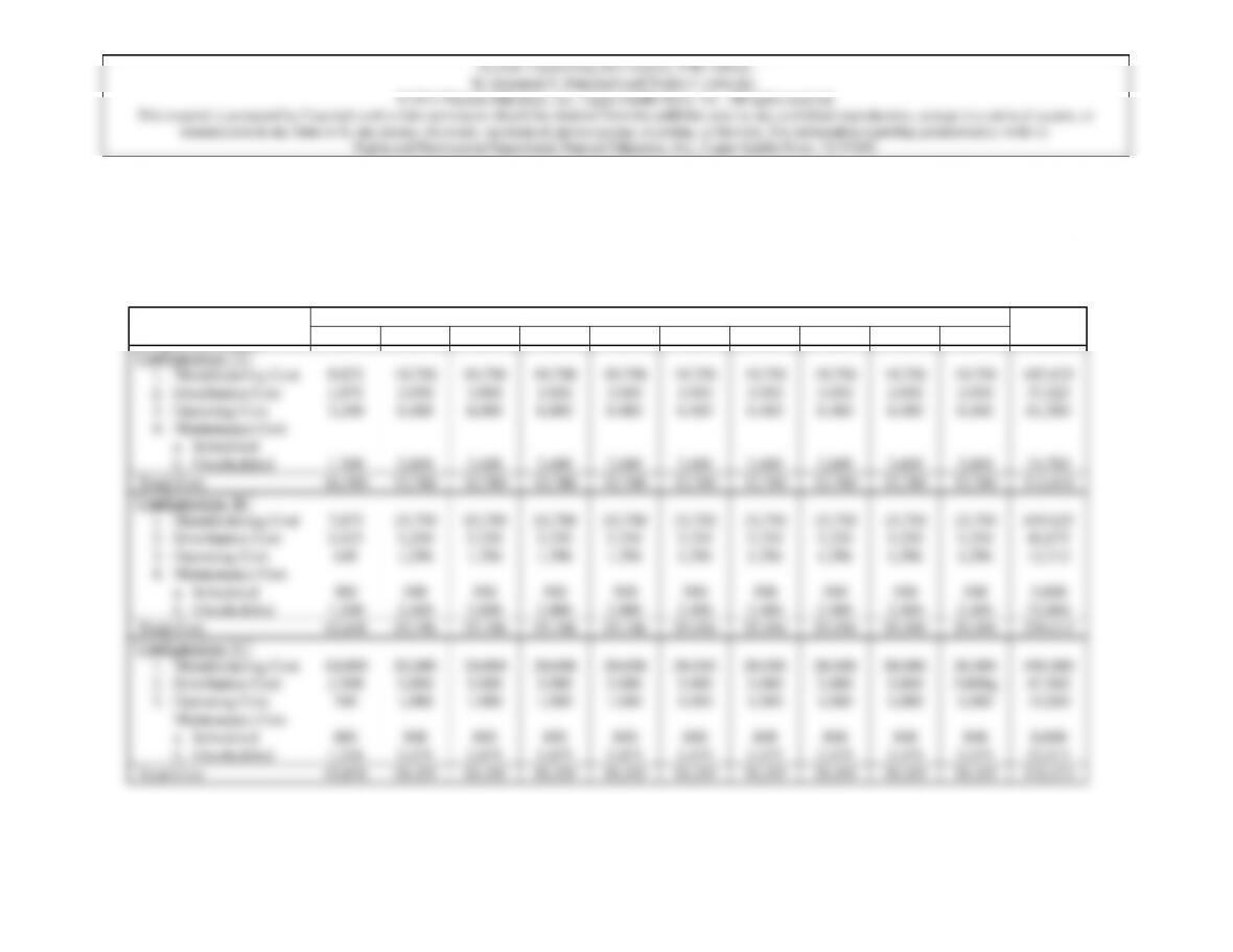
21) Table 1 exhibits the information given in this problem over a 10-year evaluation horizon.
Problem 21 – Table 1. BAF Corporation costs by program year.
Cost by Program Year ($)
Total
Evaluation Category
1
2
3
4
5
6
7
8
9
10
Cost ($)
Configuration “A”
1. Manufacturing Cost
9,875
19,750
19,750
19,750
19,750
19,750
19,750
19,750
19,750
19,750
187,625
2. Distribution Cost
1,975
3,950
3,950
3,950
3,950
3,950
3,950
3,950
3,950
3,950
37,525
3. Operating Cost
3,240
6,480
6,480
6,480
6,480
6,480
6,480
6,480
6,480
6,480
61,560
4. Maintenance Cost
a. Scheduled
b. Unscheduled
1,300
2,600
2,600
2,600
2,600
2,600
2,600
2,600
2,600
2,600
24,700
Total Cost
16,390
32,780
32,780
32,780
32,780
32,780
32,780
32,780
32,780
32,780
311,410
Configuration “B”
1. Manufacturing Cost
7,875
15,750
15,750
15,750
15,750
15,750
15,750
15,750
15,750
15,750
149,625
2. Distribution Cost
2,625
5,250
5,250
5,250
5,250
5,250
5,250
5,250
5,250
5,250
49,875
3. Operating Cost
648
1,296
1,296
1,296
1,296
1,296
1,296
1,296
1,296
1,296
12,312
4. Maintenance Cost
a. Scheduled
500
500
500
500
500
500
500
500
500
500
5,000
b. Unscheduled
1,200
2,400
2,400
2,400
2,400
2,400
2,400
2,400
2,400
2,400
22,800
Total Cost
12,848
25,196
25,196
25,196
25,196
25,196
25,196
25,196
25,196
25,196
239,612
Configuration “C”
1. Manufacturing Cost
10,000
20,000
20,000
20,000
20,000
20,000
20,000
20,000
20,000
20,000
190,000
2. Distribution Cost
2,500
5,000
5,000
5,000
5,000
5,000
5,000
5,000
5,000
5,000q
47,500
3. Operating Cost
540
1,080
1,080
1,080
1,080
1,080
1,080
1,080
1,080
1,080
10,260
Maintenance Cost
a. Scheduled
800
800
800
800
800
800
800
800
800
800
8,000
b. Unscheduled
1,238
2,475
2,475
2,475
2,475
2,475
2,475
2,475
2,475
2,475
23,513
Total Cost
15,078
29,355
29,355
29,355
29,355
29,355
29,355
29,355
29,355
29,355
279,273
Problem 21 – Table 2. Evaluation of alternative configurations for the BAF Corporation.
4
0.6830
53,957
22,389
72,715
17,209
68,300
20,049
5
0.6209
49,051
20,353
65,195
15,644
62,090
18,227
6
0.5645
44,596
18,504
59,273
14,223
56,450
16,571
7
0.5132
40,543
16,823
53,886
12,931
51,320
15,065
8
0.4665
36,854
15,292
48,983
11,754
46,650
13,694
9
0.4241
33,504
13,902
44,531
10,686
42,410
12,449
10
0.3856
30,462
12,640
40,488
9,716
38,560
11,319
Salvage
0.3505
351
—
876
—
771
—
Totals
449,875
201,524
598,845
171,597
569,786
190,397
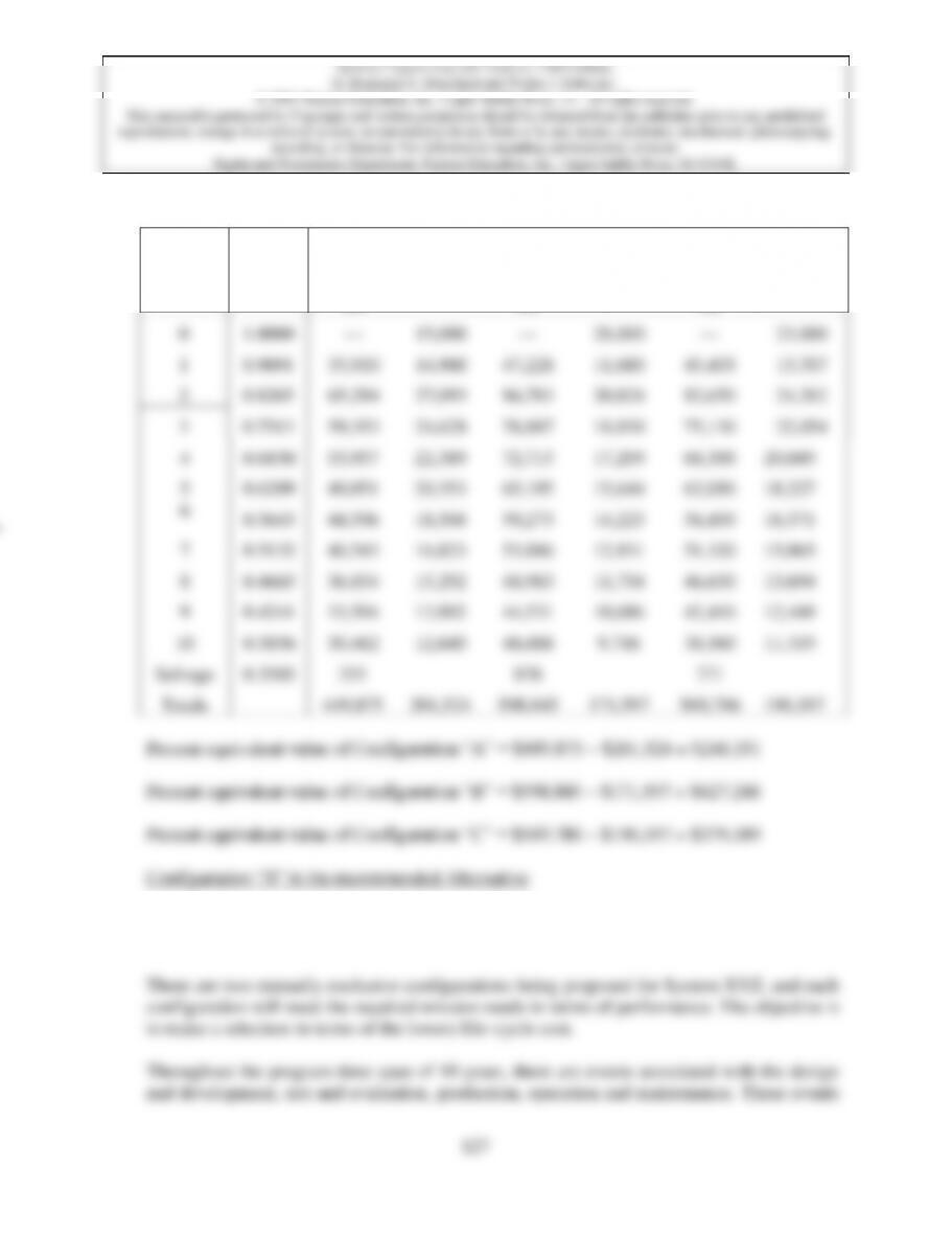
Present equivalent value of Configuration “A” = $449,875 – $201,524 = $248,351
Present equivalent value of Configuration “B” = $598,845 – $171,597 = $427,248
Present equivalent value of Configuration “C” = $569,786 – $190,397 = $379,389
Configuration “B” is the recommended Alternative
22) (a) Assume that System XYZ is “isolated” in terms of external interaction affects; address
System XYZ as an entity.
Program
year, n
(P/F,
10%,n)
Configuration “A”
Configuration “B”
Configuration “C”
Revenues
($)
Cost ($)
Revenues
($)
Cost ($)
Revenues
($)
Cost ($)
0
1.0000
—
15,000
—
28,000
—
23,000
1
0.9091
35,910
14,900
47,228
11,680
45,455
13,707
2
0.8265
65,294
27,093
86,783
20,824
82,650
24,262
3
0.7513
59,353
24,628
78,887
18,930
75,130
22,054
6

128
129
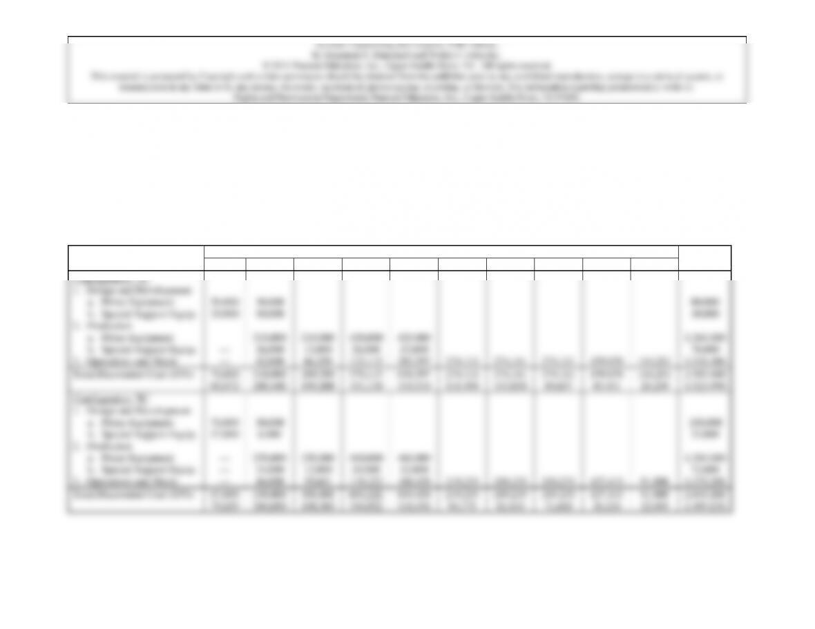
An initial step involves developing a matrix for collecting the various costs each year in terms of their inflated values. These costs are
subdivided into: 1. Design and Development; 2. Production; and 3. Operations and Maintenance as shown in the table below.
Problem 22 – Table 1. System XYZ Life Cycle Cost Summary ($)
Life–Cycle Year
Total
Item
1
2
3
4
5
6
7
8
9
10
Cost ($)
Configuration “A”
1. Design and Development
a. Prime Equipment
50,000
30,000
80,000
b. Special Support Equip.
20,000
10,000
30,000
2. Production
a. Prime Equipment
—
210,000
210,000
420,000
420,000
1,260,000
b. Special Support Equip.
—
26,000
13,000
26,000
13,000
78,000
3. Operations and Maint.
—
42,000
66,290
133,115
203,597
274,111
274,111
274,111
159,870
114,201
1,541,406
Total Discounted Cost (15%)
70,000
60,872
318,000
240,440
289,290
190,208
579,115
331,138
636,597
316,516
274,111
118,498
274,111
103,038
274,111
89,607
159,870
45,451
114,201
28,230
2,989,406
1,523,998
Configuration “B”
1. Design and Development
a. Prime Equipment
70,000
30,000
100,000
b. Special Support Equip.
17,000
6,000
23,000
2. Production
a. Prime Equipment
—
230,000
230,000
460,000
460,000
1,380,000
b. Special Support Equip.
—
24,000
12,000
24,000
12,000
72,000
3. Operations and Maint.
—
46,000
59,601
119,222
168,458
219,235
219,235
219,235
127,415
91,800
1,270,201
Total Discounted Cost (15%)
87,000
75,655
336,000
244,050
301,601
198,303
603,222
344,922
640,458
318,436
219,235
94,775
219,235
82,410
219,235
71,668
127,415
36,224
91,800
22,693
2,845,201
1,499,136
130
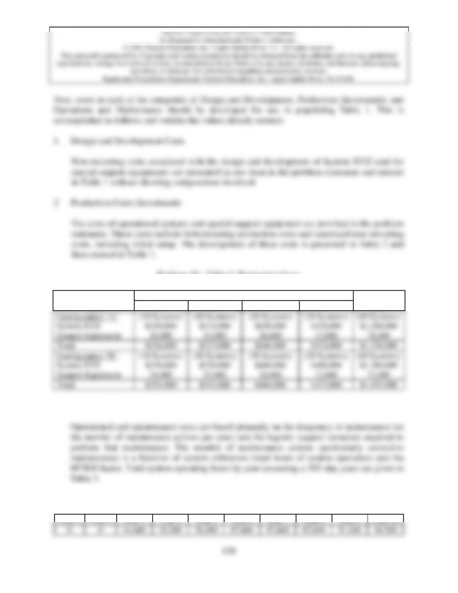
Problem 22 – Table 2. Production Costs
Year
Item
2
3
4
5
Total
Configuration “A”
(10 Systems)
(10 Systems)
(20 Systems)
(20 Systems)
(60 Systems)
System XYZ
$210,000
$210,000
$420,000
$420,000
$1,260,000
Support Equipment
26,000
13,000
26,000
13,000
78,000
Total
$236,000
$223,000
$446,000
$433,000
$1,338,000
Configuration “B”
(10 Systems)
(10 Systems)
(20 Systems)
(20 Systems)
(60 Systems)
System XYZ
$230,000
$230,000
$460,000
$460,000
$1,380,000
Support Equipment
24,000
12,000
24,000
12,000
72,000
Total
$254,000
$242,000
$484,000
$472,000
$1,452,000
3. Operations and Maintenance Costs
Problem 22 – Table 3. System Operating Hours
Year 1
Year 2
Year 3
Year 4
Year 5
Year 6
Year 7
Year 8
Year 9
Year 10
0
0
14,600
29,200
58,400
87,600
87,600
87,600
51,100
36,500
Rights and Permissions Department, Pearson Education, Inc., Upper Saddle River, NJ 07458.
131
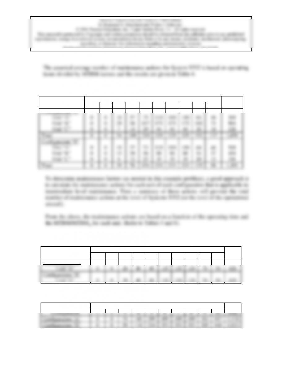
Problem 22 – Table 4. Corrective Maintenance Actions
Year
Configuration
1
2
3
4
5
6
7
8
9
10
Total
Configuration “A”
Unit “A”
0
0
18
37
73
110
110
110
64
46
568
Unit “B”
0
0
29
58
117
175
175
175
102
73
904
Unit “C”
0
0
7
14
29
44
44
44
26
18
226
Total
0
0
54
109
219
329
329
329
192
137
1,698
Configuration “B”
Unit “A”
0
0
18
37
73
110
110
110
64
46
568
Unit “B”
0
0
15
29
58
88
88
88
51
37
454
Unit “C”
0
0
6
12
23
35
35
35
20
15
181
Total
0
0
39
78
154
233
233
233
135
98
1,203
To determine maintenance factors (as needed in this example problem), a good approach is
to calculate the maintenance actions for each unit of each configuration that is applicable to
intermediate level maintenance. Then a summary of these actions will provide the total
number of maintenance actions at the level of Systems XYZ (or the level of the operational
aircraft).
From the above, the maintenance actions are based on a function of the operating time and
the MTBM/MTBMs for each unit. (Refer to Tables 5 and 6).
Problem 22 – Table 5. Preventive Maintenance Actions
Year
Configuration
1
2
3
4
5
6
7
8
9
10
Total
Configuration “A”
Unit “A”
0
0
20
40
80
120
120
120
70
50
620
Configuration “B”
Unit “A”
0
0
20
40
80
120
120
120
70
50
620
Problem 22 – Table 6. Total Maintenance Actions (Systems Level)
Year
Configuration
1
2
3
4
5
6
7
8
9
10
Total
Configuration “A”
0
0
74
149
299
499
499
499
262
187
2,318
Configuration “B”
0
0
59
118
234
353
353
353
205
148
1,823