73
CHAPTER 10
QUEUEING THEORY AND ANALYSIS
1) Monte Carlo analysis must be used in the study of a queuing system when the arrival and
service time distributions, the queuing discipline, or other system characteristics cannot be
represented mathematically. But, there is an advantage in that operational insight will be
gained from the analysis.
m
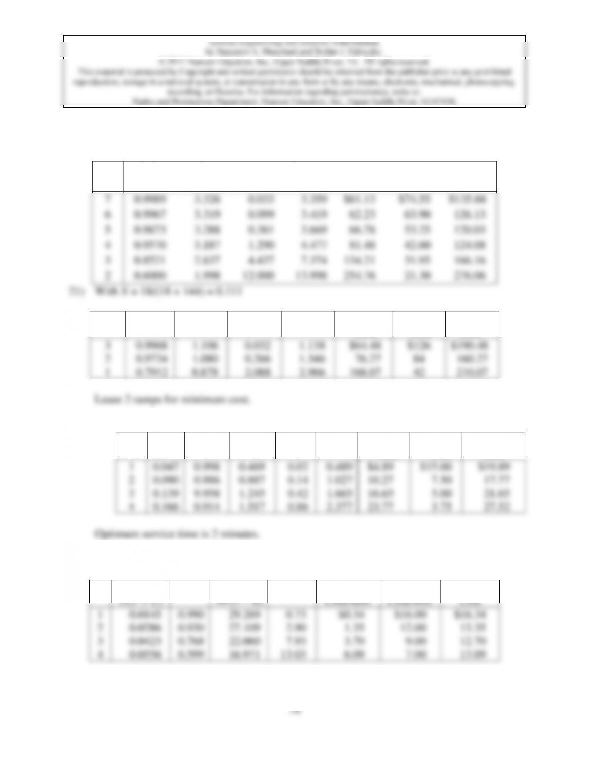
20) With X = 20/(20 + 160) = 0.111 mainimum cost is when 4 warehouse people are employed.
M
F
H
L
H+L
Waiting
Cost
Service
Cost
Total
Cost
7
0.9989
3.326
0.033
3.359
$61.13
$74.55
$135.68
6
0.9967
3.319
0.099
3.419
62.23
63.90
126.13
5
0.9873
3.288
0.381
3.669
66.78
53.25
120.03
4
0.9570
3.187
1.290
4.477
81.48
42.60
124.08
3
0.8521
2.837
4.437
7.374
134.21
31.95
166.16
2
0.6000
1.998
12.000
13.998
254.76
21.30
276.06
21) With X = 18/(18 + 144) = 0.111
M
F
H
L
H+L
Waiting
Cost
Service
Cost
Total
Cost
3
0.9968
1.106
0.032
1.138
$64.48
$126
$190.48
2
0.9734
1.080
0.266
1.346
76.27
84
160.27
1
0.7912
0.878
2.088
2.966
168.07
42
210.07
Lease 2 ramps for minimum cost.
22)
T
X
F
H
L
H+L
Waiting
Cost
Service
Cost
Total
Cost
1
0.047
0.998
0.469
0.02
0.489
$4.89
$15.00
$19.89
2
0.090
0.986
0.887
0.14
1.027
10.27
7.50
17.77
3
0.139
9.958
1.245
0.42
1.665
16.65
5.00
21.65
4
0.166
0.914
1.517
0.86
2.377
23.77
3.75
27.52
23) With N = 30, U = 68
T
X =
T/(T + U)
F
J =
NF(1 – X)
H + L
Waiting
Cost/Min.
Service
Cost/Min.
Total
Cost
1
0.0145
0.990
29.269
0.73
$0.34
$16.00
$16.34
2
0.0286
0.930
27.109
2.90
1.35
12.00
13.35
3
0.0423
0.768
22.060
7.93
3.70
9.00
12.70
4
0.0556
0.599
16.971
13.03
6.09
7.00
13.09
The minimum cost service interval is three minutes.
77
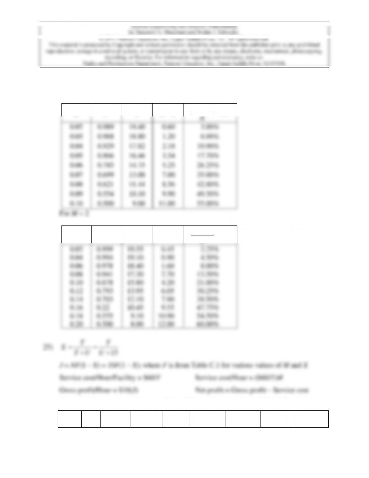
24) For M = 1
X
F
J
N – J
()
100
NJ
N
−
0.02
0.989
19.40
0.60
3.00%
0.03
0.968
18.80
1.20
6.00%
0.04
0.929
17.82
2.18
10.90%
0.05
0.866
16.46
3.54
17.70%
0.06
0.785
14.75
5.25
26.25%
0.07
0.699
13.00
7.00
35.00%
0.08
0.621
11.44
8.56
42.80%
0.09
0.554
10.10
9.90
49.50%
0.10
0.500
9.00
11.00
55.00%
For M = 2
X
F
J
N – J
()
100
NJ
N
−
0.02
0.999
19.55
0.45
2.25%
0.04
0.994
19.10
0.90
4.50%
0.06
0.978
18.40
1.60
8.00%
0.08
0.941
17.30
2.70
13.50%
0.10
0.878
15.80
4.20
21.00%
0.12
0.793
13.95
6.05
30.25%
0.14
0.703
12.10
7.90
39.50%
0.16
0.22
10.45
9.55
47.75%
0.18
0.555
9.10
10.90
54.50%
0.20
0.500
8.00
12.00
60.00%
25)
15
TT
XT U U
==
++
J = NF(1 – X) = 10F(1 – X); where F is from Table C.1 for various values of M and X
Service cost/Hour/Facility = $60/T Service cost/Hour = ($60/T)M
Gross profit/Hour = $10(J) Net profit = Gross profit – Service cost
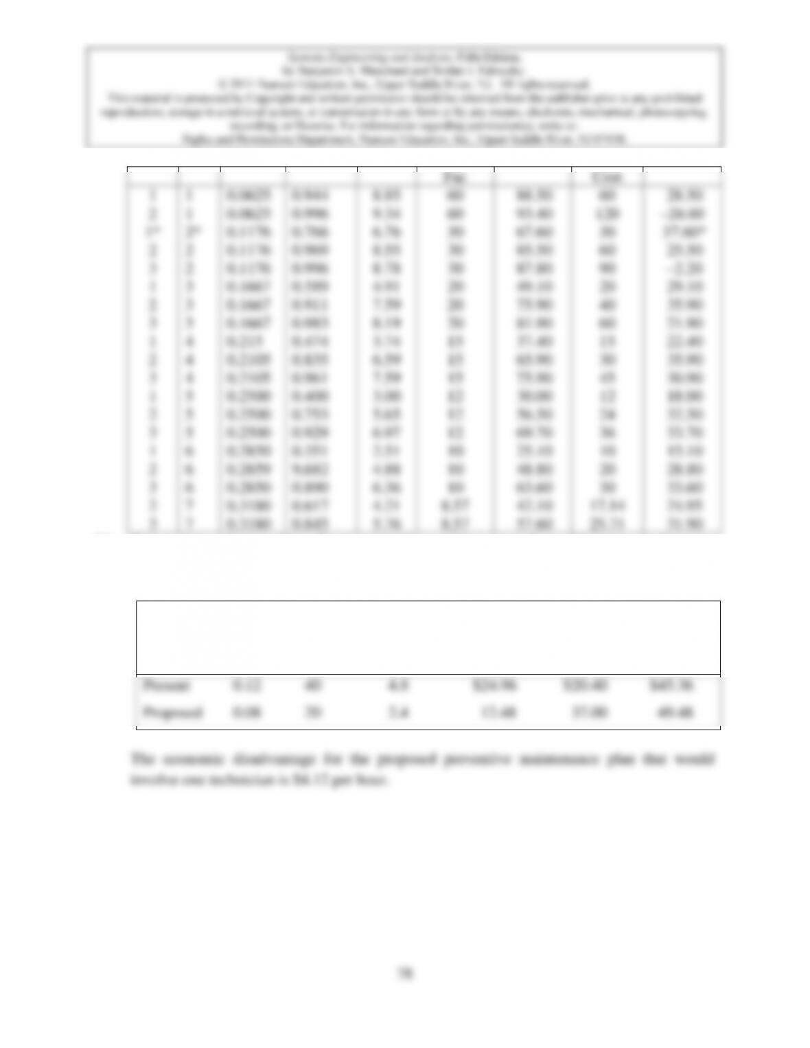
Set up a table to evaluate the net profit for different discrete values of M and T as shown:
M
T
X
F
J
Cost
Per
Gross
Profit
Total
Service
Net Profit
Fac
Cost
1
1
0.0625
0.944
8.85
60
88.50
60
28.50
2
1
0.0625
0.996
9.34
60
93.40
120
–26.60
1*
2*
0.1176
0.766
6.76
30
67.60
30
37.60*
2
2
0.1176
0.969
8.55
30
85.50
60
25.50
3
2
0.1176
0.996
8.78
30
87.80
90
–2.20
1
3
0.1667
0.589
4.91
20
49.10
20
29.10
2
3
0.1667
0.911
7.59
20
75.90
40
35.90
3
3
0.1667
0.983
8.19
20
81.90
60
21.90
1
4
0.215
0.474
3.74
15
37.40
15
22.40
2
4
0.2105
0.835
6.59
15
65.90
30
35.90
3
4
0.2105
0.961
7.59
15
75.90
45
30.90
1
5
0.2500
0.400
3.00
12
30.00
12
18.00
2
5
0.2500
0.753
5.65
12
56.50
24
32.50
3
5
0.2500
0.929
6.97
12
69.70
36
33.70
1
6
0.2850
0.351
2.51
10
25.10
10
15.10
2
6
0.2859
9,682
4.88
10
48.80
20
28.80
3
6
0.2850
0.890
6.36
10
63.60
30
33.60
2
7
0.3180
0.617
4.21
8.57
42.10
57.60
17.14
24.95
3
7
0.3180
0.845
5.76
8.57
25.71
31.90
26) Comparison of two plans for preventative maintenance, do nothing or employ one
maintenance technician.
Plan
X
% Not
Running
(Fig. 10.9)
Machines
Not
Running
Cost of
Lost
Profit
Cost of
Mechanic
Total Cost
Present
0.12
40
4.8
$24.96
$20.40
$45.36
Proposed
0.08
20
2.4
12.48
37.00
49.48