9-41
1. Fixed manufacturing overhead rate = $700,000/25,000 units = $28 per unit
2. Fixed manufacturing overhead rate = $700,000/20,000 units = $35 per unit
Manufacturing cost per unit:
$24 direct materials + $36 direct mfg. labor + $12 var. mfg. OH + $35 fixed mfg. OH = $107
3. Fixed manufacturing overhead rate = $700,000/50,000 units = $14 per unit
Manufacturing cost per unit:
of $103.20 would have been lower than the $105.00 selling price of Spirelli’s competitor, and it
would likely have resulted in higher sales. Using practical capacity will result in a higher
9-42
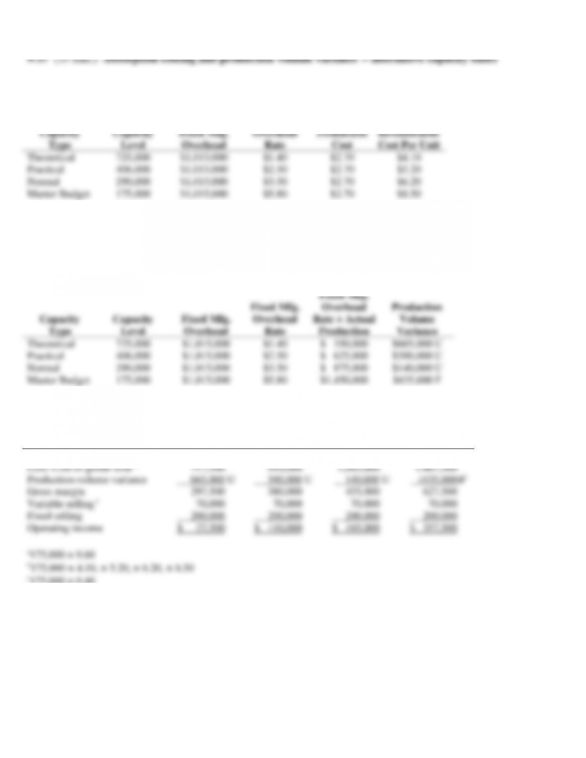
1. Inventoriable cost per unit = Variable production cost + Fixed manufacturing overhead/Capacity
Capacity
Type
Capacity
Level
Fixed Mfg.
Overhead
Fixed Mfg.
Overhead
Rate
Variable
Production
Cost
Inventoriable
Cost Per Unit
Theoretical
725,000
$1,015,000
$1.40
$2.70
$4.10
Practical
406,000
$1,015,000
$2.50
$2.70
$5.20
Normal
290,000
$1,015,000
$3.50
$2.70
$6.20
Master Budget
175,000
$1,015,000
$5.80
$2.70
$8.50
2. EBL’s actual production level is 250,000 bulbs. We can compute the production-volume variance
as:
Production Volume Variance = Budgeted Fixed Mfg. Overhead
– (Fixed Mfg. Overhead Rate × Actual Production Level)
Capacity
Type
Capacity
Level
Fixed Mfg.
Overhead
Fixed Mfg.
Overhead
Rate
Fixed Mfg.
Overhead
Rate × Actual
Production
Production
Volume
Variance
Theoretical
725,000
$1,015,000
$1.40
$ 350,000
$665,000 U
Practical
406,000
$1,015,000
$2.50
$ 625,000
$390,000 U
Normal
290,000
$1,015,000
$3.50
$ 875,000
$140,000 U
Master Budget
175,000
$1,015,000
$5.80
$1,450,000
$435,000 F
3. Operating Income for EBL given production of 250,000 bulbs and sales of 175,000 bulbs @ $9.60
apiece:
Theoretical
Practical
Normal
Master Budget
Revenue a
$1,680,000
$1,680,000
$1,680,000
$1,680,000
Less: Cost of goods sold b
717,500
910,000
1,085,000
1,487,500
Production-volume variance
665,000 U
390,000 U
140,000 U
(435,000)F
Gross margin
297,500
380,000
455,000
627,500
Variable selling c
70,000
70,000
70,000
70,000
Fixed selling
200,000
200,000
200,000
200,000
Operating income
$ 27,500
$ 110,000
$ 185,000
$ 357,500
a175,000 × 9.60
b175,000 × 4.10, × 5.20, × 6.20, × 8.50
c175,000 × 0.40
9-43
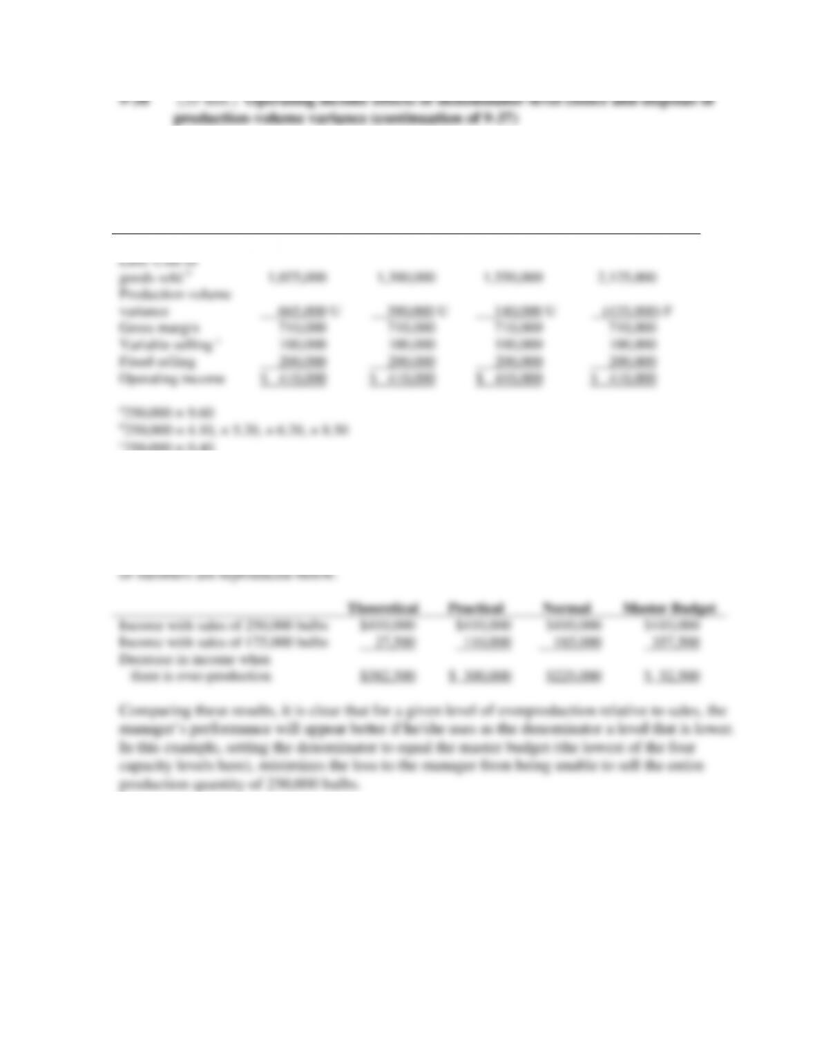
1. Since no beginning inventories exist, if EBL sells all 250,000 bulbs manufactured, its
operating income will be the same under all four capacity options. Calculations are provided
below:
Theoretical
Practical
Normal
Master Budget
Revenue a
$2,400,000
$2,400,000
$2,400,000
$2,400,000
Less: Cost of
goods sold b
1,025,000
1,300,000
1,550,000
2,125,000
Production volume
variance
665,000 U
390,000 U
140,000 U
(435,000) F
Gross margin
710,000
710,000
710,000
710,000
Variable selling c
100,000
100,000
100,000
100,000
Fixed selling
200,000
200,000
200,000
200,000
Operating income
$ 410,000
$ 410,000
$ 410,000
$ 410,000
2. If the manager of EBL produces and sells 250,000 bulbs, then all capacity levels will result in
the same operating income of $410,000 (see requirement 1 above). If the manager of EBL is
able to sell only 175,000 of the bulbs produced and if the production-volume variance is closed
to cost of goods sold, then the operating income is given as in requirement 3 of 9-37. Both sets
Income with sales of 250,000 bulbs
Income with sales of 175,000 bulbs
Decrease in income when
there is over-production
9-44
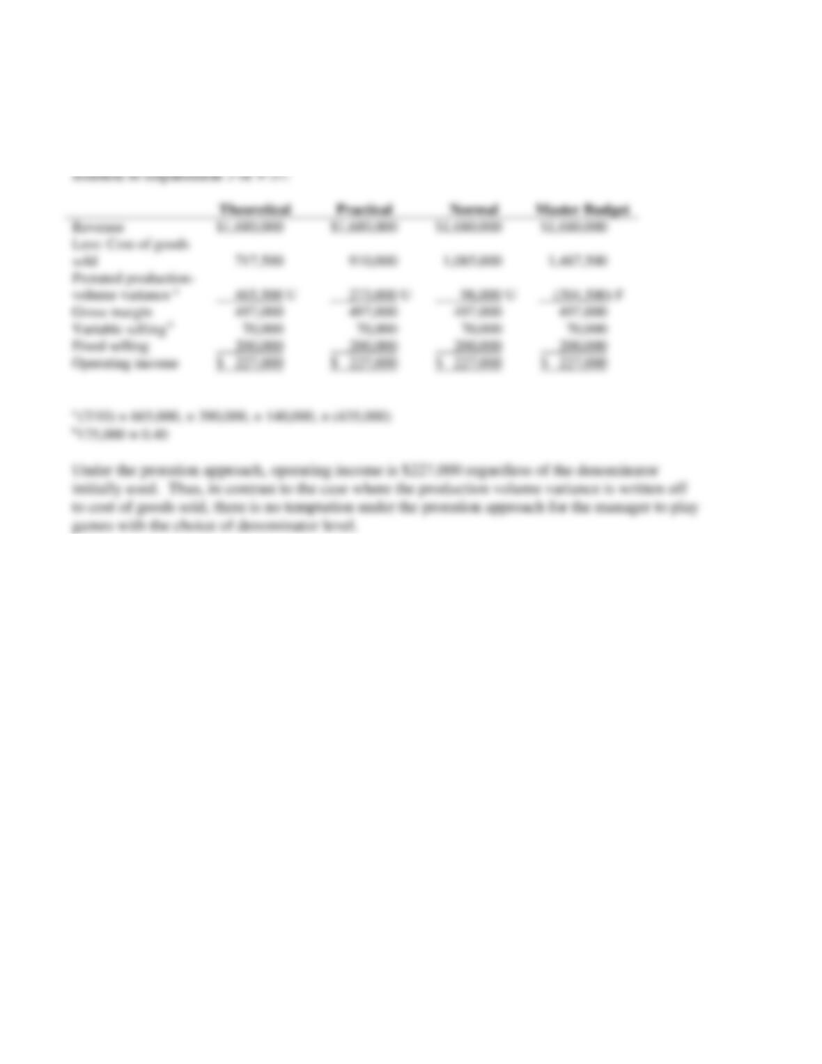
3. In this scenario, the manager of EBL produces 250,000 bulbs and sells 175,000 of them, and
the production volume variance is prorated. Given the absence of ending work in process
inventory or beginning inventory of any kind, the fraction of the production volume variance that
is absorbed into the cost of goods sold is given by 175,000/250,000 or 7/10. The operating
income under various denominator levels is then given by the following modification of the
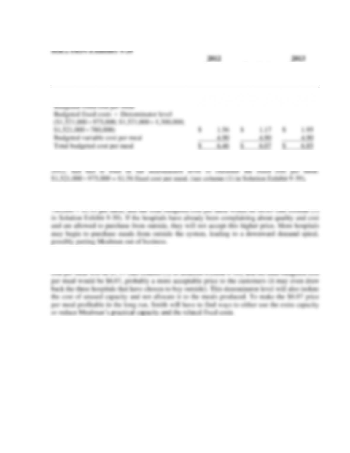
9-39 (25 min.) Cost allocation, downward demand spiral.
2012
Master
Budget
(1)
Practical
Capacity
(2)
2013
Master
Budget
(3)
Budgeted fixed costs
$1,521,000
$1,521,000
$1,521,000
Denominator level
975,000
1,300,000
780,000
Budgeted fixed cost per meal
Budgeted fixed costs
Denominator level
($1,521,000
975,000; $1,521,000
1,300,000;
$1,521,000
780,000)
$ 1.56
$ 1.17
$ 1.95
Budgeted variable cost per meal
4.90
4.90
4.90
Total budgeted cost per meal
$ 6.46
$ 6.07
$ 6.85
1. The 2012 budgeted fixed costs are $1,521,000. Mealman budgets for 975,000 meals in
2. In 2013, 3 hospitals have dropped out of the purchasing group and the master budget is
780,000 meals. If this is used as the denominator level, fixed cost per meal = $1,521,000
3. The basic problem is that Mealman has excess capacity and the associated excess fixed
costs. If Smith uses the practical capacity of 1,300,000 meals as the denominator level, the fixed
9-46
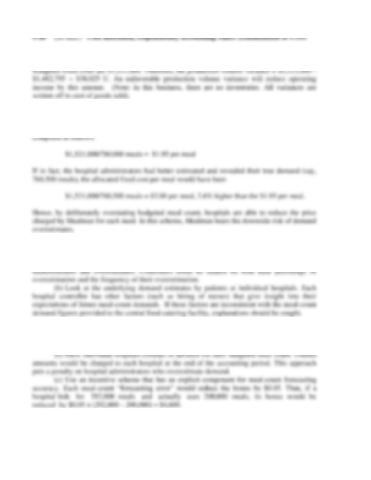
1. (See Solution Exhibit 9-39). If Mealman uses the rate based on its master budget capacity
utilization to allocate fixed costs in 2013, it would allocate 760,500
$1.95 = $1,482,975.
2. Hospitals are charged a budgeted variable cost rate and allocated budgeted fixed costs.
By overestimating budgeted meal counts, the denominator-level is larger, hence the amount
charged to individual hospitals is lower. Consider 2013 where the budgeted fixed cost rate is
3. Evidence that could be collected include:
(a) Budgeted meal-count estimates and actual meal-count figures each year for each
hospital controller. Over an extended time period, there should be a sizable number of both
4. (a) Highlight the importance of a corporate culture of honesty and openness. Cayzer
could institute a Code of Ethics that highlights the upside of individual hospitals providing
honest estimates of demand (and the penalties for those who do not).