9-21
1. a, b
2. a
3. d
4. c, d
5. c
6. d
7. a
9. b
10. c, d
11. a, b
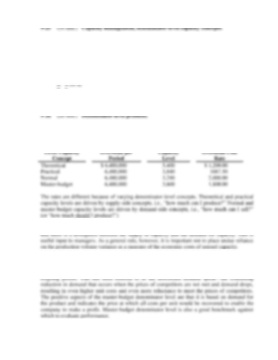
1. Budgeted fixed manufacturing overhead costs rates:
Denominator
Level Capacity
Concept
Budgeted Fixed
Manufacturing
Overhead per
Period
Budgeted
Capacity
Level
Budgeted Fixed
Manufacturing
Overhead Cost
Rate
Theoretical
$ 6,480,000
5,400
$ 1,200.00
Practical
6,480,000
3,840
1687.50
Normal
6,480,000
3,240
2,000.00
Master-budget
6,480,000
3,600
1,800.00
The rates are different because of varying denominator-level concepts. Theoretical and practical
capacity levels are driven by supply-side concepts, i.e., “how much can I produce?” Normal and
master-budget capacity levels are driven by demand–side concepts, i.e., “how much can I sell?”
(or “how much should I produce?”)
2. The variances that arise from use of the theoretical or practical level concepts will signal
3. Under a cost-based pricing system, the choice of a master-budget level denominator will
lead to high prices when demand is low (more fixed costs allocated to the individual product
level), further eroding demand; conversely, it will lead to low prices when demand is high,
9-22
1.
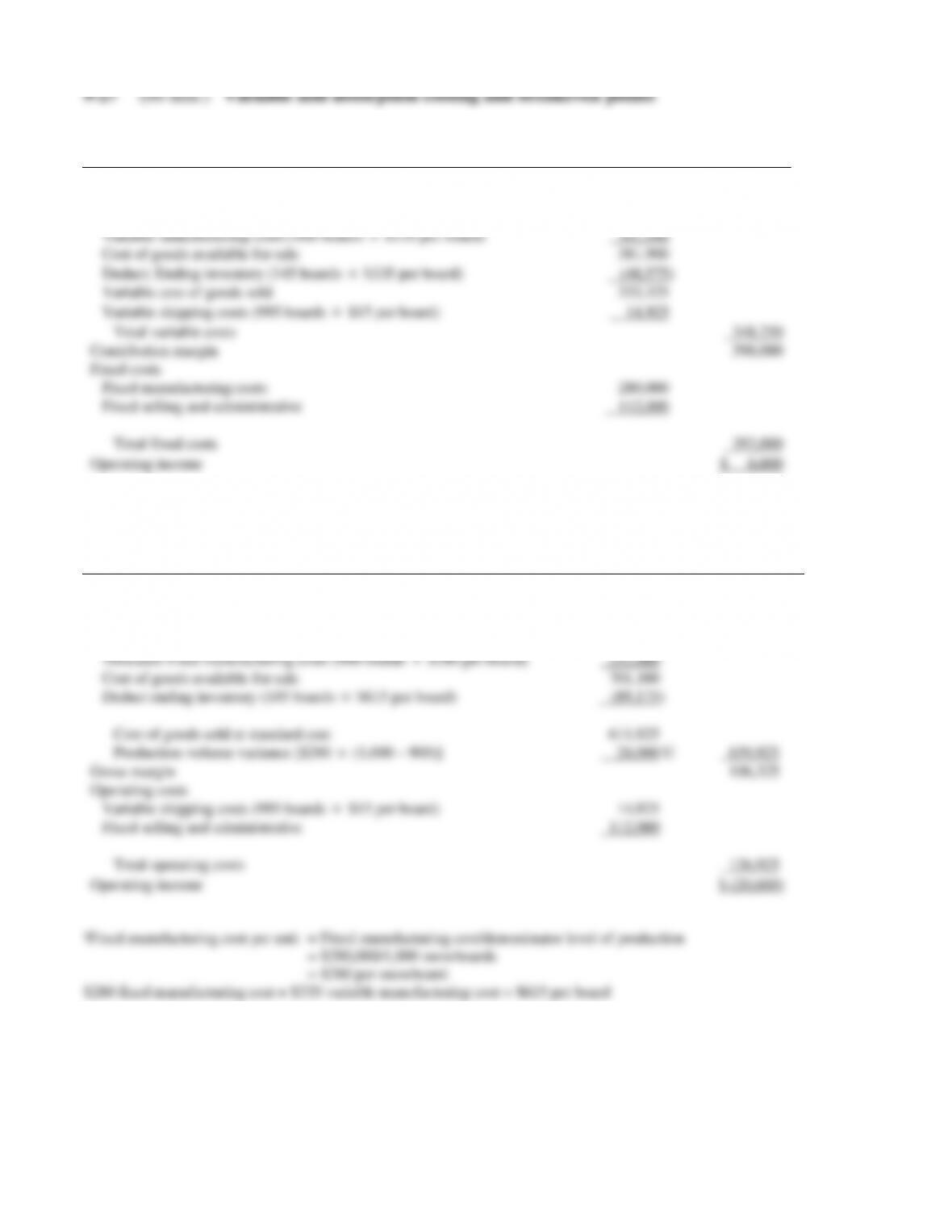
2011 Variable-Costing Based Operating Income Statement
Revenues (995 boards
$750 per board)
$746,250
Variable costs
Beginning inventory (240 boards
$335 per board)
$ 80,400
Variable manufacturing costs (900 boards
$335 per board)
301,500
Cost of goods available for sale
381,900
Deduct: Ending inventory (145 boards
$335 per board)
(48,575)
Variable cost of goods sold
333,325
Variable shipping costs (995 boards
$15 per board)
14,925
Total variable costs
348,250
Contribution margin
398,000
Fixed costs
Fixed manufacturing costs
280,000
Fixed selling and administrative
112,000
Total fixed costs
392,000
Operating income
$ 6,000
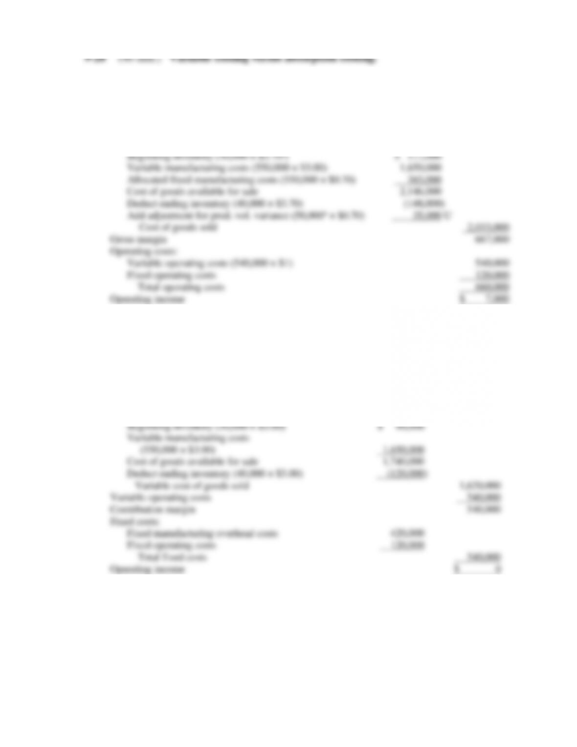
2.
2011 Absorption-Costing Based Operating Income Statement
Revenues (995 boards
$750 per board)
$746,250
Cost of goods sold
Beginning inventory (240 boards
$615a per board)
$147,600
Variable manufacturing costs (900 boards
$335 per board)
301,500
Allocated fixed manufacturing costs (900 boards
$280 per board)
252,000
Cost of goods available for sale
701,100
Deduct ending inventory (145 boards
$615 per board)
(89,175)
Cost of goods sold at standard cost
611,925
Production-volume variance [$280
(1,000 – 900)]
28,000 U
639,925
Gross margin
106,325
Operating costs
Variable shipping costs (995 boards
$15 per board)
14,925
Fixed selling and administrative
112,000
Total operating costs
126,925
Operating income
$ (20,600)
9-23
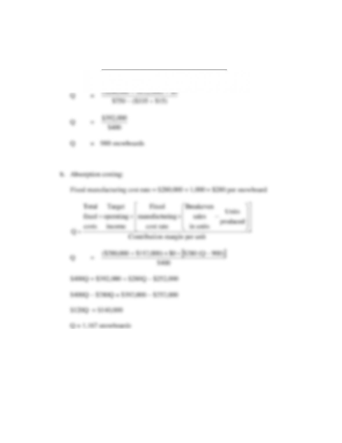
3. Breakeven point in units:
a. Variable Costing:
Q =
Total Fixed Costs Target Operating Income
Contribution Margin Per Unit
+
0$)000,112$000,280($
++
9-24
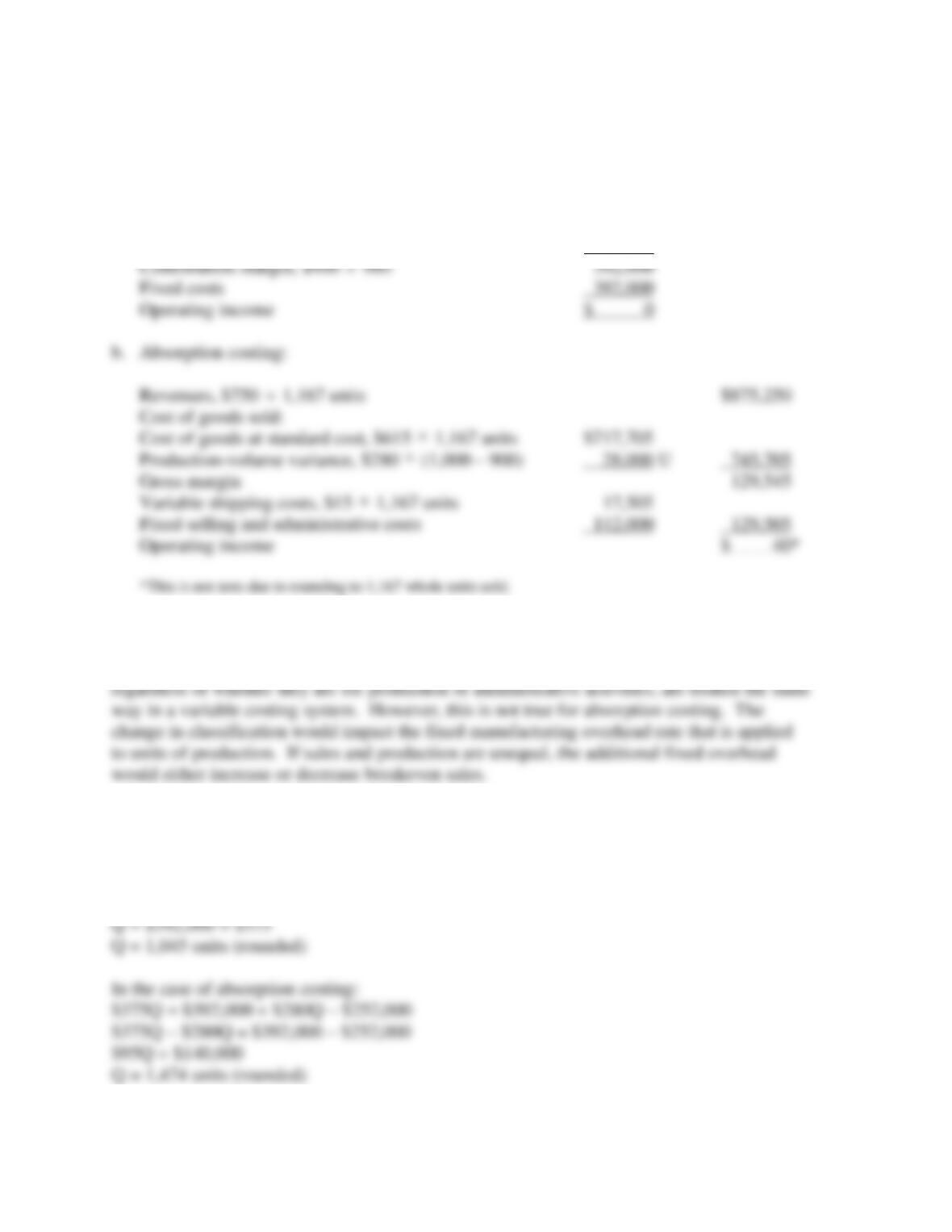
4. Proof of breakeven point:
a. Variable Costing:
Revenues, $750
980 units $735,000
Variable costs, $350
980 343,000
5. If $20,000 of fixed administrative costs were reclassified as production costs, there would
be no change in breakeven sales using variable costing. This is because all fixed costs,
6. The additional $25 per unit variable production cost will cause unit contribution margin
to decrease from $400 to $375. This decrease will cause the breakeven point to increase.
In the case of variable costing:
9-25
1. Absorption Costing: Mavis Company Income Statement
For the Year Ended December 31, 2012
Revenues (540,000 × $5.00) $2,700,000
Cost of goods sold:
a $3.00 + ($7.00 ÷ 10) = $3.00 + $0.70 = $3.70
b [(10 units per mach. hr. × 60,000 mach. hrs.) – 550,000 units)] = 50,000 units unfavorable
2. Variable Costing: Mavis Company Income Statement
For the Year Ended December 31, 2012
Revenues $2,700,000
Variable cost of goods sold:
9-26
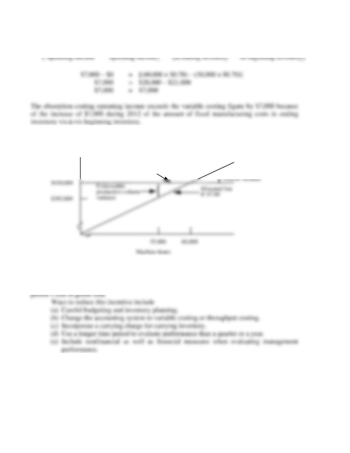
3. The difference in operating income between the two costing methods is:
( ) ( )
Absorption costing Variable costing Fixed manuf. costs Fixed manuf. costs
operating income operating income in ending inventory in beginning inventory
− = −
4.
Total fixed manufacturing costs
$420,000
$385,000
Actual and budget line
Unfavorable
production-volume
variance
{
Allocated line
@ $7.00
55,000
60,000
Machine-hours
}
Favorable production-
volume variance
5. Absorption costing is more likely to lead to buildups of inventory than does variable
costing. Absorption costing enables managers to increase reported operating income by building
up inventory which reduces the amount of fixed manufacturing overhead included in the current
9-27
1. The treatment of fixed manufacturing overhead in absorption costing is affected primarily
by what denominator level is selected as a base for allocating fixed manufacturing costs to units
produced. In this case, is 20,000 tons per year, 40,000 tons, or some other denominator level the
most appropriate base?
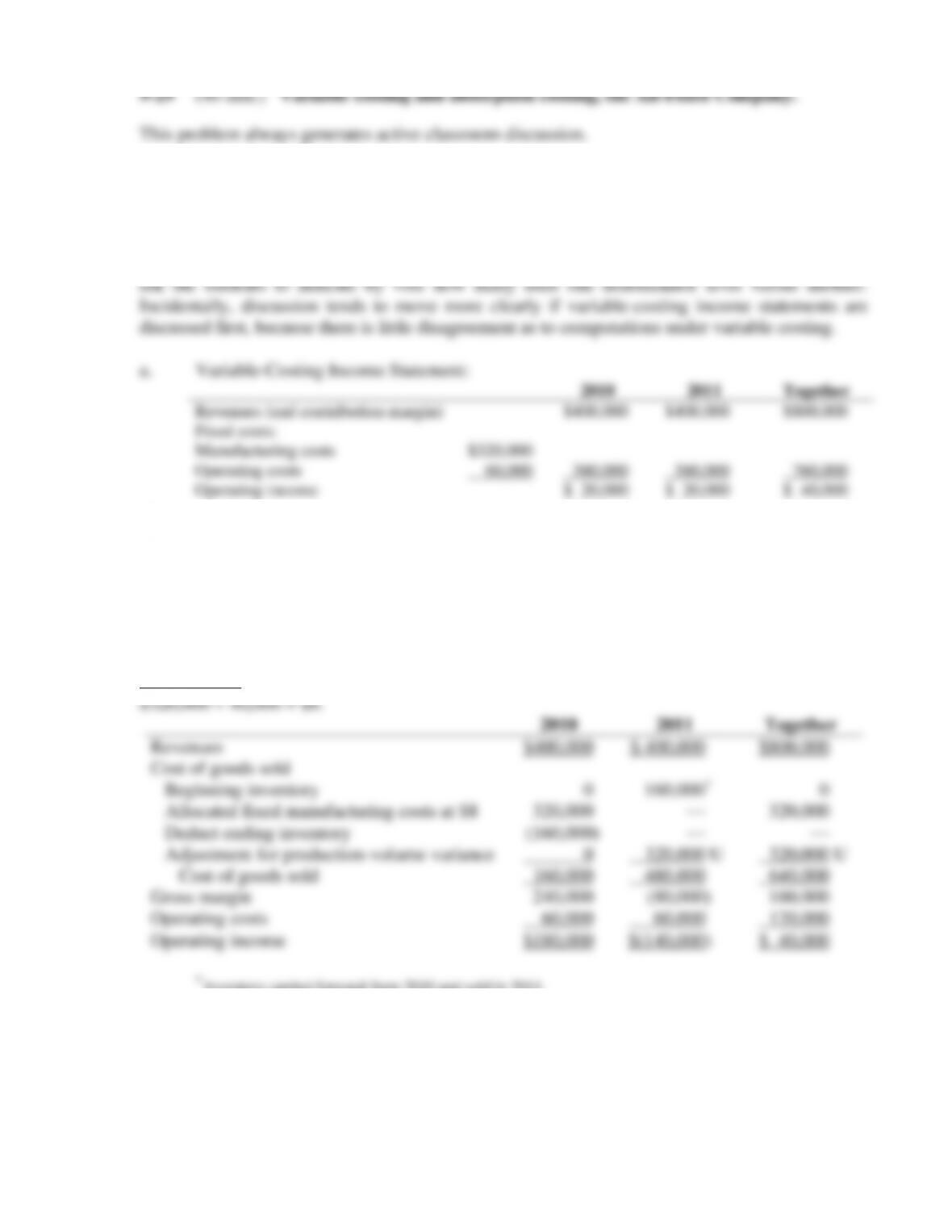
We usually place the following possibilities on the board or overhead projector and then
2010
2011
Together
Revenues (and contribution margin)
$400,000
$400,000
$800,000
Fixed costs:
Manufacturing costs
$320,000
Operating costs
60,000
380,000
380,000
760,000
Operating income
$ 20,000
$ 20,000
$ 40,000
b. Absorption-Costing Income Statement:
The ambiguity about the 20,000- or 40,000-unit denominator level is intentional. IF YOU WISH,
THE AMBIGUITY MAY BE AVOIDED BY GIVING THE STUDENTS A SPECIFIC
DENOMINATOR LEVEL IN ADVANCE.
Alternative 1. Use 40,000 units as a denominator; fixed manufacturing overhead per unit is
9-28
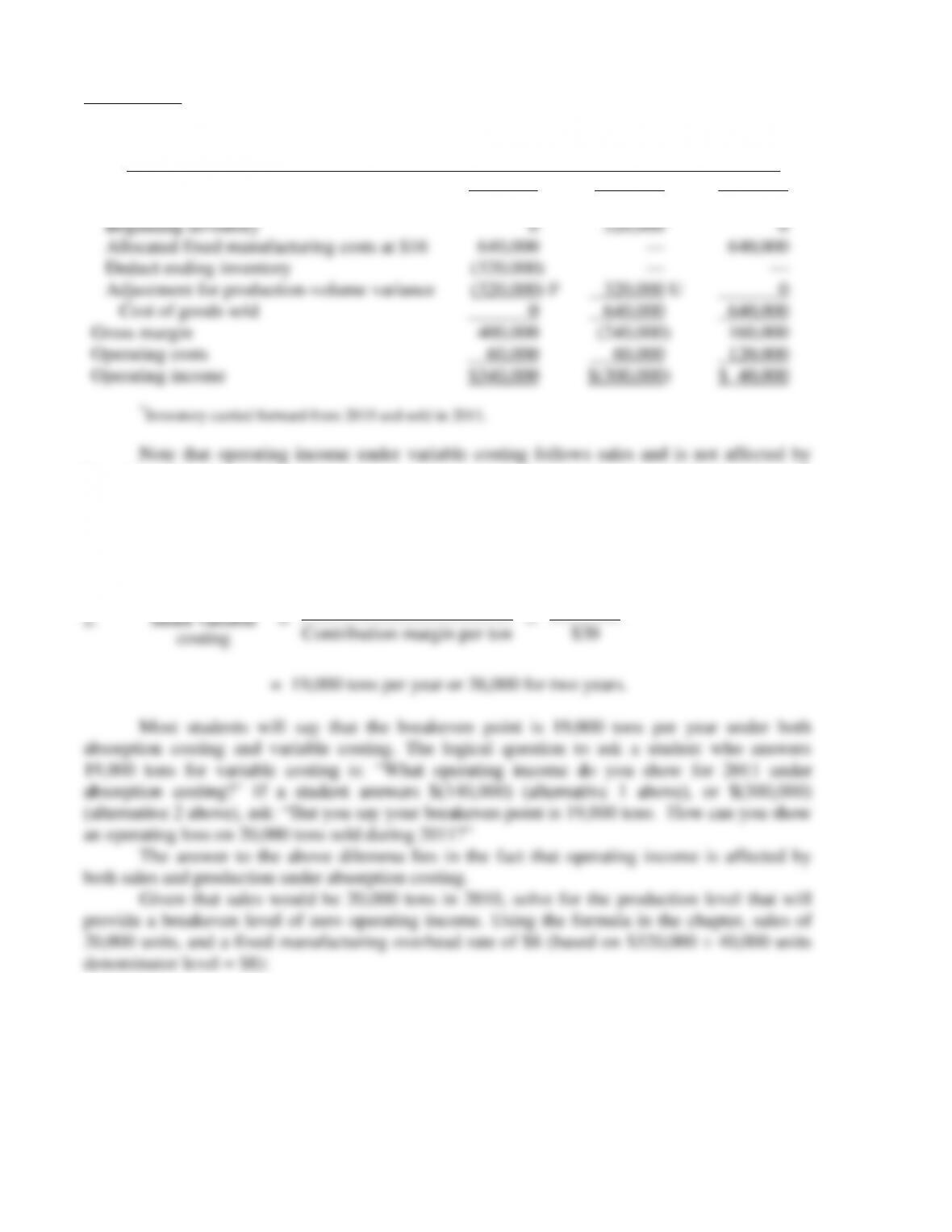
Alternative 2. Use 20,000 units as a denominator; fixed manufacturing overhead per unit is
$320,000 20,000 = $16.
2010
2011
Together
Revenues
$400,000
$400,000
$800,000
Cost of goods sold
Beginning inventory
0
320,000*
0
Allocated fixed manufacturing costs at $16
640,000
—
640,000
Deduct ending inventory
(320,000)
—
—
Adjustment for production-volume variance
(320,000) F
320,000 U
0
Cost of goods sold
0
640,000
640,000
Gross margin
400,000
(240,000)
160,000
Operating costs
60,000
60,000
120,000
Operating income
$340,000
$(300,000)
$ 40,000
inventory changes.
Note also that students will understand the variable-costing presentation much more
easily than the alternatives presented under absorption costing.
Breakeven point
costing
Fixed costs $380,000
Contribution margin per ton $20
= 19,000 tons per year or 38,000 for two years.
Most students will say that the breakeven point is 19,000 tons per year under both
absorption costing and variable costing. The logical question to ask a student who answers
19,000 tons for variable costing is: “What operating income do you show for 2011 under
absorption costing?” If a student answers $(140,000) (alternative 1 above), or $(300,000)
(alternative 2 above), ask: “But you say your breakeven point is 19,000 tons. How can you show
an operating loss on 20,000 tons sold during 2011?”
The answer to the above dilemma lies in the fact that operating income is affected by
both sales and production under absorption costing.
Given that sales would be 20,000 tons in 2010, solve for the production level that will
provide a breakeven level of zero operating income. Using the formula in the chapter, sales of
20,000 units, and a fixed manufacturing overhead rate of $8 (based on $320,000 ÷ 40,000 units
denominator level = $8):
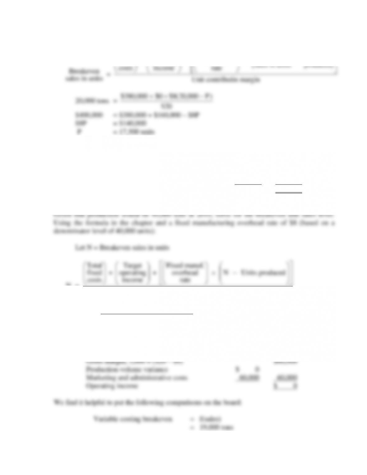
Let P = Production level
Breakeven
sales in units
=
( )
Total Target Fixed manuf. Breakeven Units
fixed + operating + overhead
sales in units produced
costs income rate
Unit contributin margin
−
20,000 tons =
20$
)000‚20(8$0$000‚380$P−++
$400,000 = $380,000 + $160,000 – $8P
$8P = $140,000
P = 17,500 units
Proof:
Gross margin, 20,000 × ($20 – $8) $240,000
Production-volume variance,
(40,000 – 17,500) × $8 $180,000
Marketing and administrative costs 60,000 240,000
Operating income $ 0
N
=
Total Target Fixed manuf.
fixed + operating + overhead N Units produced
costs income rate
Unit contributin margin
−
N =
20$
)000,40(8$0$000‚380$ −++ N
$20N = $380,000 + $8N – $320,000
$12N = $60,000
N = 5,000
Proof:
9-30
Absorption costing breakeven = f(sales and production)
3. Absorption costing inventory cost: Either $160,000 (using 40,000 denominator level) or
4. Operating income is affected by both production and sales under absorption costing.