8-41
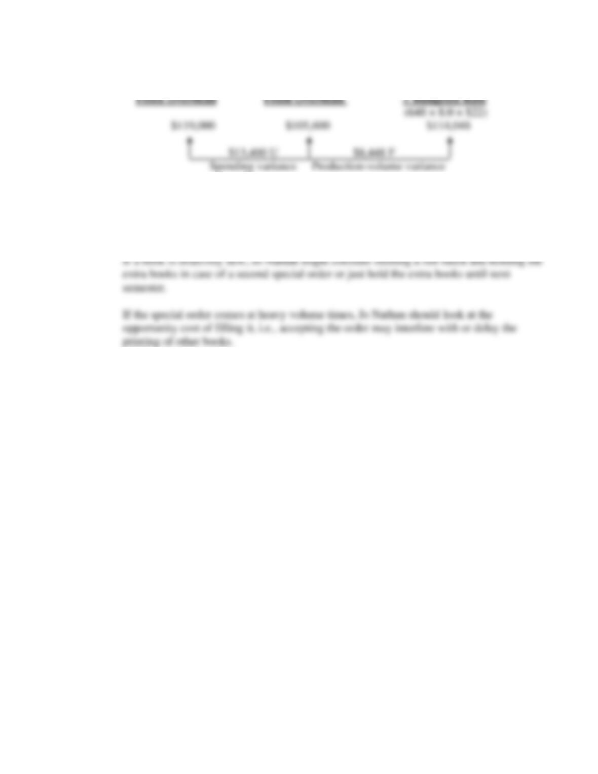
7. Fixed Setup Overhead Variance Analysis for Jo Nathan Publishing Company for 2012
Actual Static Budget Standard Hours
8. Rejecting an order may have implications for future orders (i.e., professors would be
reluctant to order books from this publisher again). Jo Nathan should consider factors
such as prior history with the customer and potential future sales.
8-42
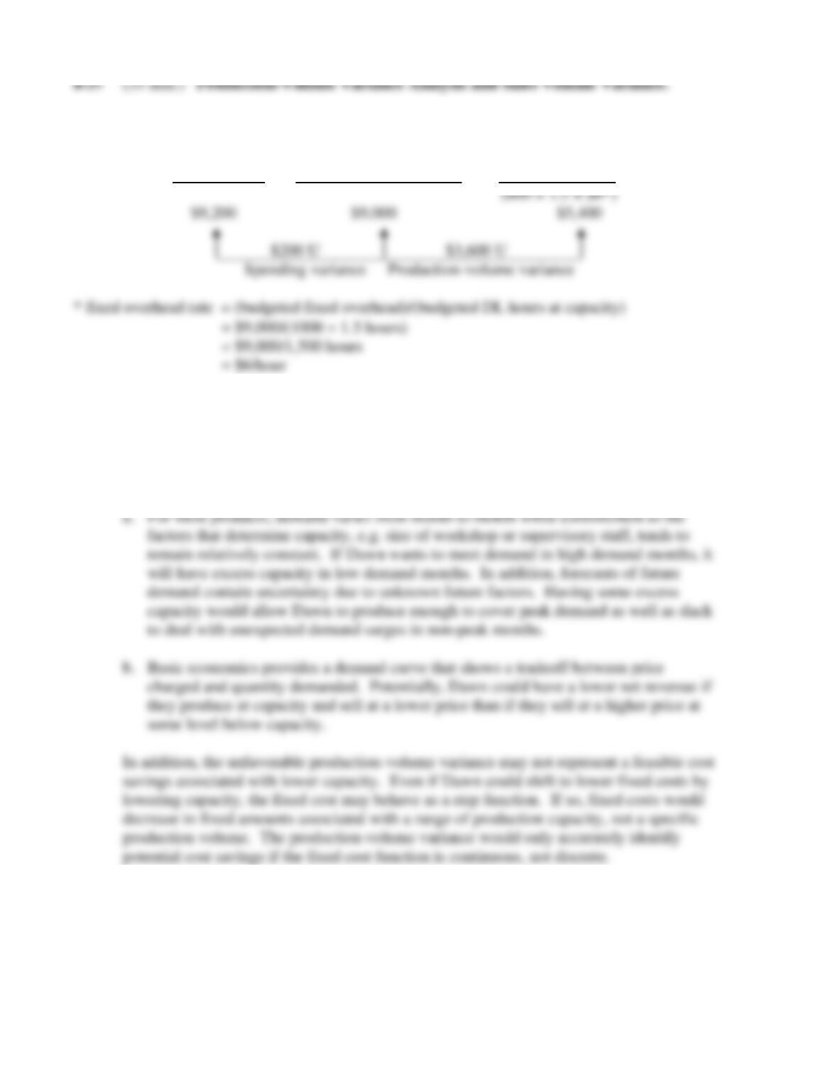
1. and 2. Fixed Overhead Variance Analysis for Dawn Floral Creations, Inc. for February
Actual Fixed Static Budget Standard Hours
Overhead Fixed Overhead × Budgeted Rate
3. An unfavorable production-volume variance measures the cost of unused capacity. Production
at capacity would result in a production-volume variance of 0 since the fixed overhead rate is
based upon expected hours at capacity production. However, the existence of an unfavorable
volume variance does not necessarily imply that management is doing a poor job or incurring
unnecessary costs. Using the suggestions in the problem, two reasons can be identified.
8-43
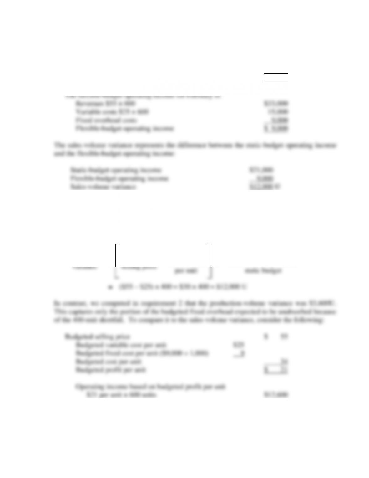
4. The static-budget operating income for February is:
Revenues $55 × 1,000 $55,000
Variable costs $25 × 1,000 25,000
Fixed overhead costs 9,000
Static-budget operating income $21,000
Equivalently, the sales-volume variance captures the fact that when Dawn sells 600 units instead
of the budgeted 1,000, only the revenue and the variable costs are affected. Fixed costs remain
unchanged. Therefore, the shortfall in profit is equal to the budgeted contribution margin per
unit times the shortfall in output relative to budget.
Sales-volume
variable cost
units sold relative to the
8-44
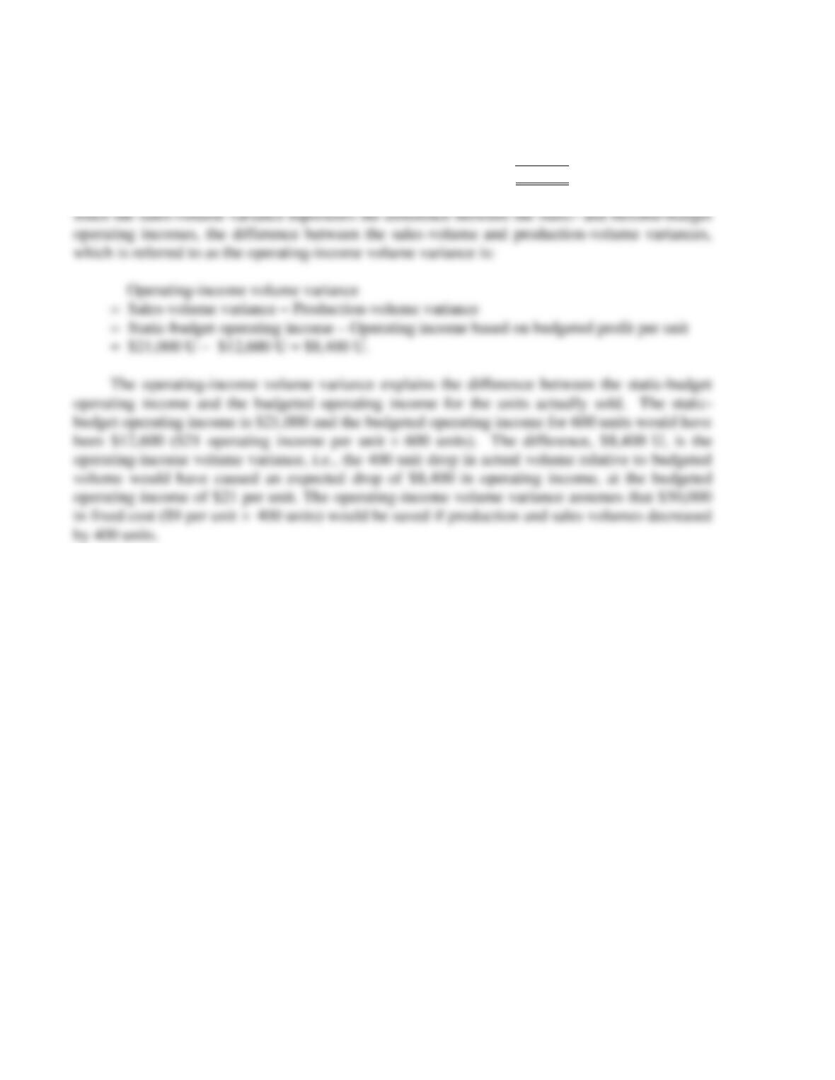
The $3,600 U production-volume variance explains the difference between operating income
based on the budgeted profit per unit and the flexible-budget operating income:
Operating income based on budgeted profit per unit $12,600
Production-volume variance 3,600 U
Flexible-budget operating income $ 9,000
8-45
8-38 (30−40 min.) Comprehensive review of Chapters 7 and 8, working backward from
given variances.
1. Solution Exhibit 8-38 outlines the Chapter 7 and 8 framework underlying this solution.
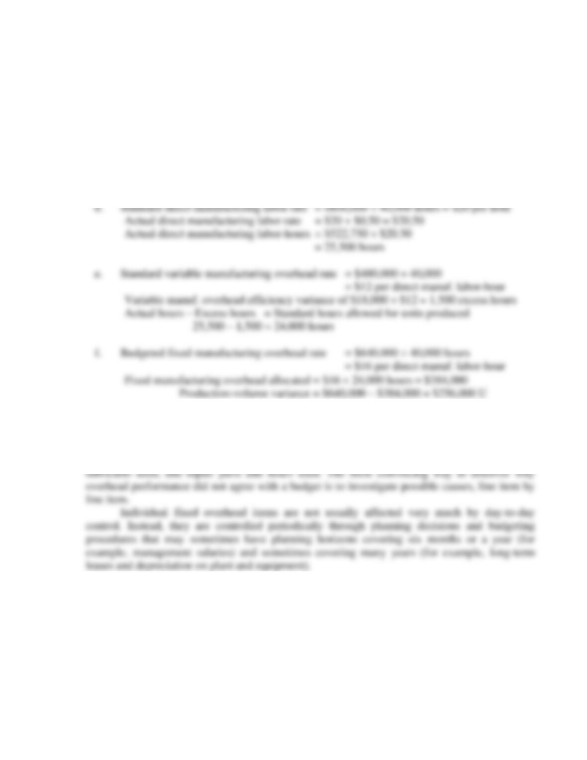
a. Pounds of direct materials purchased = $176,000 ÷ $1.10 = 160,000 pounds
b. Pounds of excess direct materials used = $69,000 ÷ $11.50 = 6,000 pounds
c. Variable manufacturing overhead spending variance = $10,350 – $18,000 = $7,650 F
2. The control of variable manufacturing overhead requires the identification of the cost drivers
for such items as energy, supplies, and repairs. Control often entails monitoring nonfinancial
measures that affect each cost item, one by one. Examples are kilowatts used, quantities of
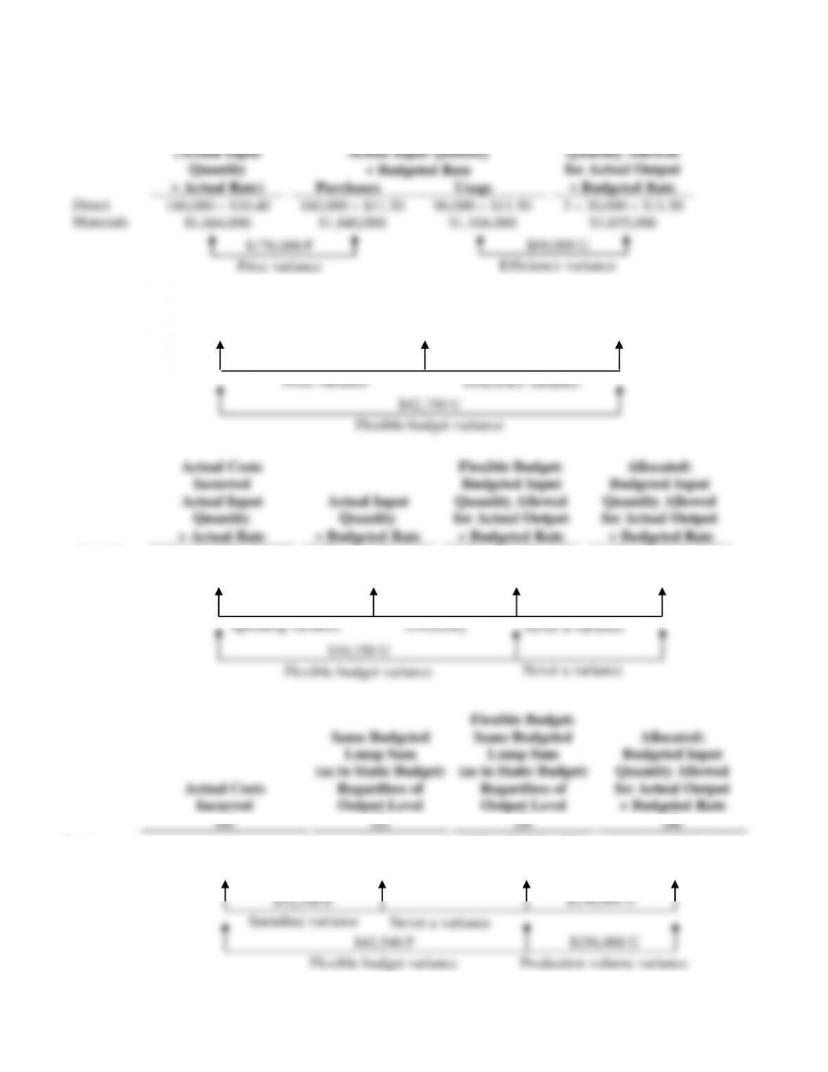
SOLUTION EXHIBIT 8-38
Actual Costs
Incurred
(Actual Input
Quantity
Actual Rate)
Actual Input Quantity
Budgeted Rate
Purchases Usage
Flexible Budget:
Budgeted Input
Quantity Allowed
for Actual Output
Budgeted Rate
Direct
Materials
160,000 $10.40
$1,664,000
160,000 $11.50
$1,840,000
96,000 $11.50
$1,104,000
3 30,000 $11.50
$1,035,000
Direct
Manuf.
Labor
0.85 30,000 $20.50
$522,750
0.85 30,000 $20
$510,000
0.80 30,000 $20
$480,000
$176,000 F
Price variance
$69,000 U
Efficiency variance
$12,750 U
Price variance
$30,000 U
Efficiency variance
Quantity
Budgeted Rate
Variable
0.80 30,000 $12
8-47
8-39 (30−50 min.) Review of Chapters 7 and 8, 3-variance analysis.
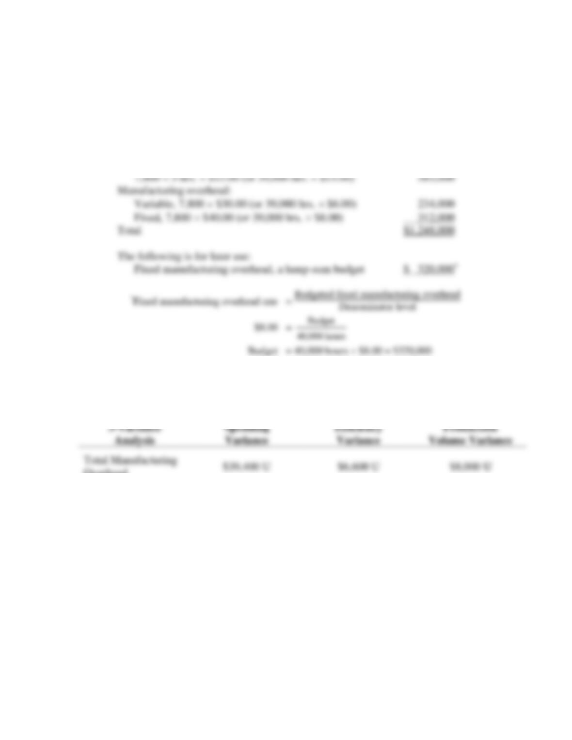
1. Total standard production costs are based on 7,800 units of output.
Direct materials, 7,800 $15.00
7,800 3 lbs. $5.00 (or 23,400 lbs. $5.00) $ 117,000
Direct manufacturing labor, 7,800 $75.00
2. Solution Exhibit 8-39 presents a columnar presentation of the variances. An overview of
the 3-variance analysis using the block format of the text is:
3-Variance
Analysis
Spending
Variance
Efficiency
Variance
Production
Volume Variance
Total Manufacturing
Overhead
$39,400 U
$6,600 U
$8,000 U